| << Chapter < Page | Chapter >> Page > |
Sketch the graph of

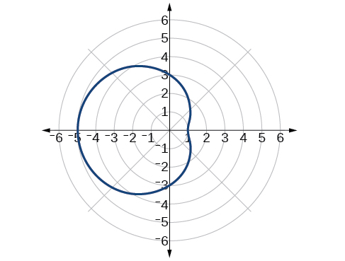
Another type of limaçon, the inner-loop limaçon , is named for the loop formed inside the general limaçon shape. It was discovered by the German artist Albrecht Dürer (1471-1528), who revealed a method for drawing the inner-loop limaçon in his 1525 book Underweysung der Messing . A century later, the father of mathematician Blaise Pascal , Étienne Pascal(1588-1651), rediscovered it.
The formulas that generate the inner-loop limaçons are given by and where and The graph of the inner-loop limaçon passes through the pole twice: once for the outer loop, and once for the inner loop. See [link] for the graphs.

Sketch the graph of
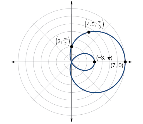
Testing for symmetry, we find that the graph of the equation is symmetric about the polar axis. Next, finding the zeros reveals that when The maximum is found when or when Thus, the maximum is found at the point (7, 0).
Even though we have found symmetry, the zero, and the maximum, plotting more points will help to define the shape, and then a pattern will emerge.
See [link] .
| 7 | 6.3 | 4.5 | 2 | −0.5 | −2.3 | −3 | −2.3 | −0.5 | 2 | 4.5 | 6.3 | 7 |
As expected, the values begin to repeat after The graph is shown in [link] .

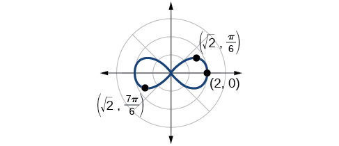
The lemniscate is a polar curve resembling the infinity symbol or a figure 8. Centered at the pole, a lemniscate is symmetrical by definition.
The formulas that generate the graph of a lemniscate are given by and where The formula is symmetric with respect to the pole. The formula is symmetric with respect to the pole, the line and the polar axis. See [link] for the graphs.

Sketch the graph of
The equation exhibits symmetry with respect to the line the polar axis, and the pole.
Let’s find the zeros. It should be routine by now, but we will approach this equation a little differently by making the substitution
So, the point is a zero of the equation.
Now let’s find the maximum value. Since the maximum of when the maximum when Thus,
We have a maximum at (2, 0). Since this graph is symmetric with respect to the pole, the line and the polar axis, we only need to plot points in the first quadrant.
Make a table similar to [link] .
| 0 | |||||
| 2 | 0 | 0 |
Plot the points on the graph, such as the one shown in [link] .

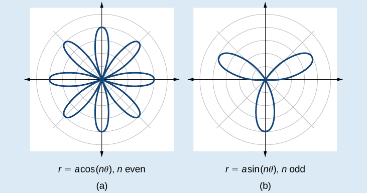
The next type of polar equation produces a petal-like shape called a rose curve. Although the graphs look complex, a simple polar equation generates the pattern.
The formulas that generate the graph of a rose curve are given by and where If is even, the curve has petals. If is odd, the curve has petals. See [link] .


Notification Switch
Would you like to follow the 'Essential precalculus, part 2' conversation and receive update notifications?