| << Chapter < Page | Chapter >> Page > |
Based on the Taylor expansion of K (- τ , Γ) about τ = 0, the logarithm of g 1 ( τ ) is given as [link] .
Importantly, if look back at the Seigert relationship in the logarithmic form, [link] .
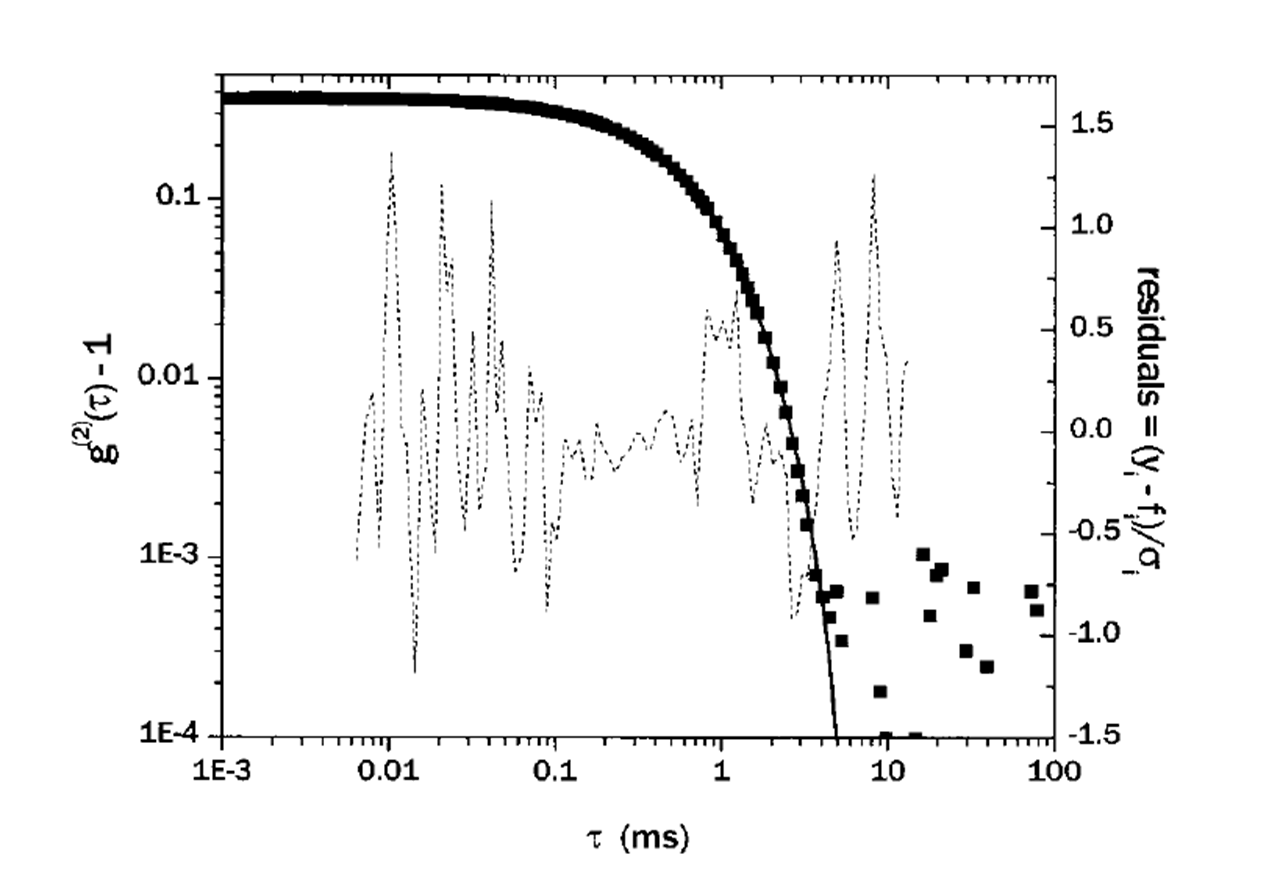
The measured data of g 2 ( τ ) could be fitted with the parameters of k m using the relationship of [link] , where ( k 1 ), k 2 , and k 3 describes the average, variance, and skewness (or asymmetry) of the decay rates of the distribution, and polydispersity index is used to indicate the width of the distribution. And parameters beyond k 3 are seldom used to prevent overfitting the data. Finally, the size distribution can be easily calculated from the decay rate distribution as described in [link] . [link] shows an example of data fitting using the cumulant method.

When using the cumulant expansion method however, one should keep in mind that it is only suitable for monomodal distributions (Gaussian-like distribution centered about the mean), and for non-monomodal distributions, other methods like exponential sampling and CONTIN regularization should be applied instead.
Now that the size distribution is able to be acquired from the fluctuation data of the scattered light using cumulant expansion or other methods, it is worthwhile to understand the three kinds of distribution index usually used in size analysis: number weighted distribution, volume weighted distribution, and intensity weighted distribution.
First of all, based on all the theories discussed above, it should be clear that the size distribution given by DLS experiments is the intensity weighted distribution, as it is always the intensity of the scattering that is being analyzed. So for intensity weighted distribution, the contribution of each particle is related to the intensity of light scattered by that particle. For example, using Rayleigh approximation, the relative contribution for very small particles will be proportional to a 6 .
For number weighted distribution, given by image analysis as an example, each particle is given equal weighting irrespective of its size, which means proportional to a 0 . This index is most useful where the absolute number of particles is important, or where high resolution (particle by particle) is required.
For volume weighted distribution, given by laser diffraction as an example, the contribution of each particle is related to the volume of that particle, which is proportional to a 3 . This is often extremely useful from a commercial perspective as the distribution represents the composition of the sample in terms of its volume/mass, and therefore its potential money value.

Notification Switch
Would you like to follow the 'Physical methods in chemistry and nano science' conversation and receive update notifications?