| << Chapter < Page | Chapter >> Page > |
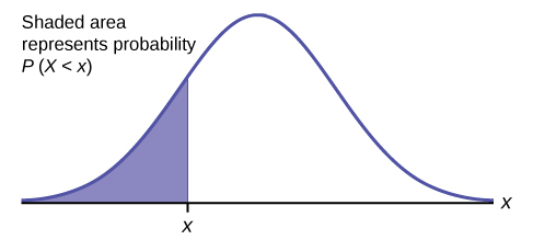
The shaded area in the following graph indicates the area to the left of x . This area is represented by the probability P ( X < x ). Normal tables, computers, and calculators provide or calculate the probability P ( X < x ).

The area to the right is then P ( X > x ) = 1 – P ( X < x ). Remember, P ( X < x ) = Area to the left of the vertical line through x . P ( X < x ) = 1 – P ( X < x ) = Area to the right of the vertical line through x . P ( X < x ) is the same as P ( X ≤ x ) and P ( X > x ) is the same as P ( X ≥ x ) for continuous distributions.
Probabilities are calculated using technology.
To calculate the probability, you can use probability tables without the use of technology.
If the area to the left is 0.0228, then the area to the right is 1 – 0.0228 = 0.9772.
If the area to the left of x is 0.012, then what is the area to the right?
1 − 0.012 = 0.988
The final exam scores in a statistics class were normally distributed with a mean of 63 and a standard deviation of five.
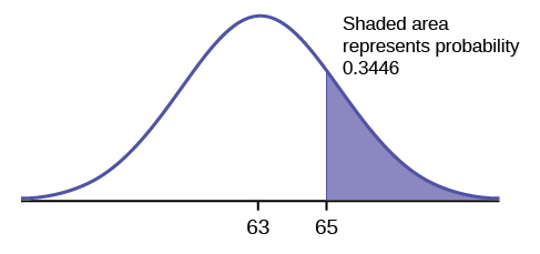
a. Find the probability that a randomly selected student scored more than 65 on the exam.
a. Let X = a score on the final exam. X ~ N (63, 5), where μ = 63 and σ = 5
Draw a graph.
Then, find P ( x >65).
P ( x >65) = 0.3446

The probability that any student selected at random scores more than 65 is 0.3446.
Before technology, the z -score was looked up in a standard normal probability table (because the math involved is too cumbersome) to find the probability. In this example, a standard normal table with area to the left of the z -score was used. You calculate the z -score and look up the area to the left. The probability is the area to the right.
z = = 0.4
Area to the left is 0.6554.
P ( x >65) = P ( z >0.4) = 1 – 0.6554 = 0.3446
b. Find the probability that a randomly selected student scored less than 85.
b. Draw a graph.
Then find P ( x <85), and shade the graph.
Using a computer or calculator, find P ( x <85) = 1.
The probability that one student scores less than 85 is approximately one (or 100%).
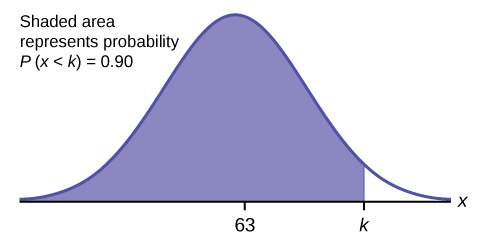
c. Find the 90 th percentile (that is, find the score k that has 90% of the scores below k and 10% of the scores above k ).
c. Find the 90 th percentile. For each problem or part of a problem, draw a new graph. Draw the x -axis. Shade the area that corresponds to the 90 th percentile.
Let k = the 90 th percentile. The variable k is located on the x -axis. P ( x < k ) is the area to the left of k . The 90 th percentile k separates the exam scores into those that are the same or lower than k and those that are the same or higher. Ninety percent of the test scores are the same or lower than k , and ten percent are the same or higher. The variable k is often called a critical value .
k = 69.4

The 90 th percentile is 69.4. This means that 90% of the test scores fall at or below 69.4 and 10% fall at or above.
d. Find the 70 th percentile (that is, find the score k such that 70% of scores are below k and 30% of the scores are above k ).
d. Find the 70 th percentile.
Draw a new graph and label it appropriately. k = 65.6
The 70 th percentile is 65.6. This means that 70% of the test scores fall at or below 65.5 and 30% fall at or above.

Notification Switch
Would you like to follow the 'Statistics i - math1020 - red river college - version 2015 revision a - draft 2015-10-24' conversation and receive update notifications?