<< Chapter < Page Chapter >> Page >
  • Recognize the format of a double integral over a polar rectangular region.
  • Evaluate a double integral in polar coordinates by using an iterated integral.
  • Recognize the format of a double integral over a general polar region.
  • Use double integrals in polar coordinates to calculate areas and volumes.

Double integrals are sometimes much easier to evaluate if we change rectangular coordinates to polar coordinates. However, before we describe how to make this change, we need to establish the concept of a double integral in a polar rectangular region.

Polar rectangular regions of integration

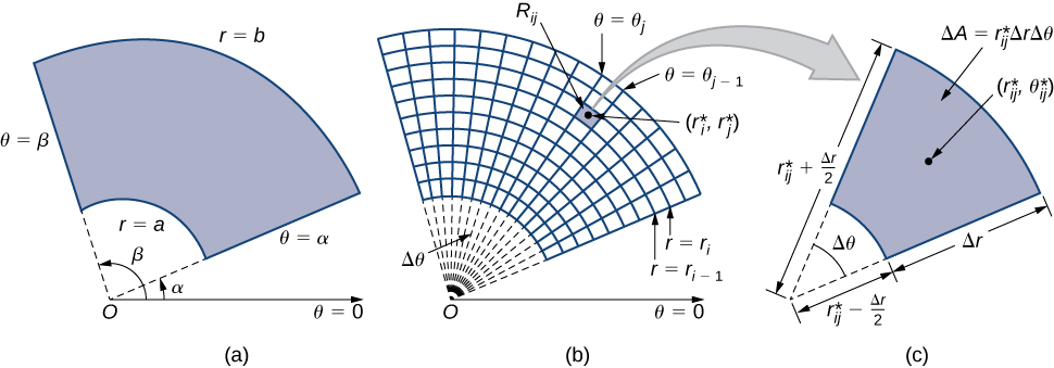
When we defined the double integral for a continuous function in rectangular coordinates—say, g over a region R in the x y -plane—we divided R into subrectangles with sides parallel to the coordinate axes. These sides have either constant x -values and/or constant y -values. In polar coordinates, the shape we work with is a polar rectangle    , whose sides have constant r -values and/or constant θ -values. This means we can describe a polar rectangle as in [link] (a), with R = { ( r , θ ) | a r b , α θ β } .

In this section, we are looking to integrate over polar rectangles. Consider a function f ( r , θ ) over a polar rectangle R . We divide the interval [ a , b ] into m subintervals [ r i 1 , r i ] of length Δ r = ( b a ) / m and divide the interval [ α , β ] into n subintervals [ θ i 1 , θ i ] of width Δ θ = ( β α ) / n . This means that the circles r = r i and rays θ = θ i for 1 i m and 1 j n divide the polar rectangle R into smaller polar subrectangles R i j ( [link] (b)).

This figure consists of three figures labeled a, b, and c. In figure a, a sector of an annulus is shown in the polar coordinate plane with radii a and b and angles alpha and beta from the theta = 0 axis. In figure b, this sector of an annulus is cut up into subsectors in a manner similar to the way in which previous spaces were cut up into subrectangles. In figure c, one of these subsectors is shown with angle Delta theta, distance between inner and outer radii Delta r, and area Delta A = r* sub theta Delta r Delta theta, where the center point is given as (r* sub i j, theta* sub i j).
(a) A polar rectangle R (b) divided into subrectangles R i j . (c) Close-up of a subrectangle.

As before, we need to find the area Δ A of the polar subrectangle R i j and the “polar” volume of the thin box above R i j . Recall that, in a circle of radius r , the length s of an arc subtended by a central angle of θ radians is s = r θ . Notice that the polar rectangle R i j looks a lot like a trapezoid with parallel sides r i 1 Δ θ and r i Δ θ and with a width Δ r . Hence the area of the polar subrectangle R i j is

Δ A = 1 2 Δ r ( r i 1 Δ θ + r 1 Δ θ ) .

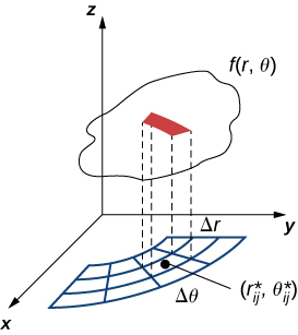
Simplifying and letting r i j * = 1 2 ( r i 1 + r i ) , we have Δ A = r i j * Δ r Δ θ . Therefore, the polar volume of the thin box above R i j ( [link] ) is

f ( r i j * , θ i j * ) Δ A = f ( r i j * , θ i j * ) r i j * Δ r Δ θ .
In x y z space, there is a surface f (r, theta). On the x y plane, a series of subsectors of annuli are drawn as in the previous figure with radius between annuli Delta r and angle between subsectors Delta theta. A subsector from the surface f(r, theta) is projected down onto one of these subsectors. This subsector has center point marked (r* sub i j, theta* sub i j).
Finding the volume of the thin box above polar rectangle R i j .

Using the same idea for all the subrectangles and summing the volumes of the rectangular boxes, we obtain a double Riemann sum as

i = 1 m j = 1 n f ( r i j * , θ i j * ) r i j * Δ r Δ θ .

As we have seen before, we obtain a better approximation to the polar volume of the solid above the region R when we let m and n become larger. Hence, we define the polar volume as the limit of the double Riemann sum,

V = lim m , n i = 1 m j = 1 n f ( r i j * , θ i j * ) r i j * Δ r Δ θ .

This becomes the expression for the double integral.

Definition

The double integral of the function f ( r , θ ) over the polar rectangular region R in the r θ -plane is defined as

R f ( r , θ ) d A = lim m , n i = 1 m j = 1 n f ( r i j * , θ i j * ) Δ A = lim m , n i = 1 m j = 1 n f ( r i j * , θ i j * ) r i j * Δ r Δ θ .

Again, just as in Double Integrals over Rectangular Regions , the double integral over a polar rectangular region can be expressed as an iterated integral in polar coordinates. Hence,

R f ( r , θ ) d A = R f ( r , θ ) r d r d θ = θ = α θ = β r = a r = b f ( r , θ ) r d r d θ .
Practice Key Terms 1

Get Jobilize Job Search Mobile App in your pocket Now!

Get it on Google Play Download on the App Store Now


Source:  OpenStax, Calculus volume 3. OpenStax CNX. Feb 05, 2016 Download for free at http://legacy.cnx.org/content/col11966/1.2
Google Play and the Google Play logo are trademarks of Google Inc.

Notification Switch

Would you like to follow the 'Calculus volume 3' conversation and receive update notifications?

Ask