| << Chapter < Page | Chapter >> Page > |
For each currency, k and week t , , , . Estimates were based on a moving 26 week window of data. For example, were estimated from and (when volatility covariates were included). The partial log-likelihood function is
Parameters, were estimated using a version of the Nelder and Mead algorithm on the penalized problem:
The penalization ensures the constraint is maintained in the solution.
The α s where initialized with the quantiles of the distribution I could not use a data based initialization such as the method of moments to initialize the optimization since ξ s are not observed. . Table 1 lists initial and estimated value of for each k .
For each 26 week window, the lag order l k of each currency k was determined by building nested models and comparing adjacent models using the partial likelihood ratio test.
For example, at , we wish to estimate the lag for . Models to be tested are,
Due to the computation time required to compute the lag for each window (parameters up to lag seven had to be estimated) for each window (over all instruments). On my pc it took over 10 hours. , I chose to keep the lag order of each instrument fixed to that obtained from the first window, ([ ]).These estimates are shown in Table 2. Since when volatility is included as predictor, I set .
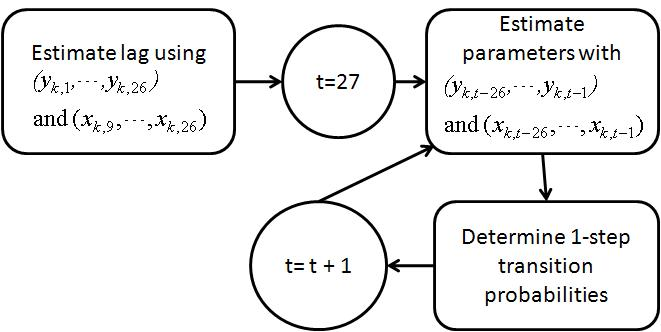
With the lags estimated from the first six months, the appropriate model , , , for each instrument is identified. Then, after each week t , the one-step transition probability estimates , are estimated by estimating parameters ( , , ) from the past 26 weeks of rank and volatility data then estimate using model . Finally estimate
. These steps are summarized in Figure 1.

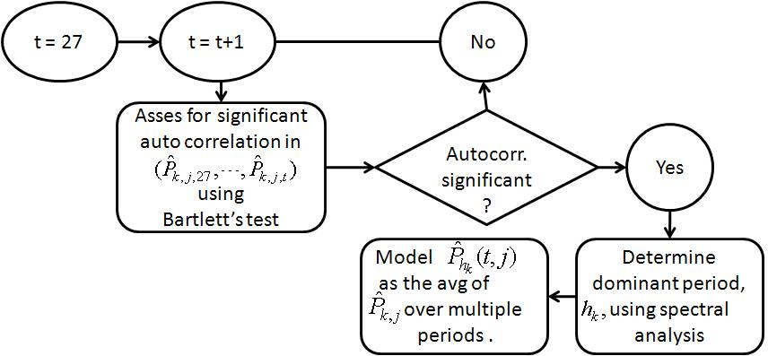
For the periodic transition probability model let represent the transition probability of currency k being in ranking j at week t. Obtain from , as follows. Estimate h k as the dominant frequency obtained from spectral analysis of . Suppose the sequence is of length N . Let
Then for some week t , if , then
The flow chart in Figure 2 summarizes the steps followed to obtain the estimates.

Figures 3, 4, 5 and 6 show the estimated transition probabilities for YEN and the AUD from week 27 to week 127. From Figures 5 and 6 we observe that for AUD, on average and tend to have lowest value over the most weeks than any of the other ranking categories. This result matches intuition; if a currency has higher odds of yielding the most (least) return over a long period, more market players will buy (sell) the instrument exerting an upward (downward) pressure on its price thereby reshuffling rankings (and ranking probabilities). However, the estimated transition probabilities for the YEN contradict this assumption (see Figure 5). tended to be much higher on average than , which tended to be least. Overall, Figures 36 highlight two shortcomings: the requirements:

Notification Switch
Would you like to follow the 'The art of the pfug' conversation and receive update notifications?