0.11 Decision trees  (Page 5/5)

The dyadic decision trees studied here are different than classical tree rules, such as CART orC4.5. Those techniques select a tree according to

for some $\alpha >0$ whereas ours was roughly

for $\alpha \approx \sqrt{\frac{3log2}{2n}}$ . The square root penalty is essential for the risk bound. No such bound exists for CARTor C4.5. Moreover, recent experimental work has shown that the square root penalty often performs better in practice. Finally,recent results show that a slightly tighter bounding procedure for the estimation error can be used to show thatdyadic decision trees (with a slightly different pruning procedure) achieve a rate of

which turns out to be the minimax optimal rate (i.e., under the boundary assumptions above, no method can achieve a faster rate of convergence tothe Bayes error).

Box counting dimension

The notion of dimension of a sets arises in many aspects of mathematics, and it is particularly relevant to the study offractals (that besides some important applications make really cool t-shirts). The dimension somehow indicates how we shouldmeasure the contents of a set (length, area, volume, etc...). The box-counting dimension is a simple definition of the dimension ofa set. The main idea is to cover the set with boxes with sidelength $r$ . Let $N\left(r\right)$ denote the smallest number of such boxes, then the box counting dimension is defined as

Although the boxes considered above do not need to be aligned on a rectangulargrid (and can in fact overlap) we can usually consider them over a grid and obtain an upper bound on the box-counting dimension. Toillustrate the main ideas let's consider a simple example, and connect it to the classification scenario considered before.

Let $f:[0,1]\to [0,1]$ be a Lipschitz function, with Lipschitz constant $L$ ( i.e., $\left|f\right(a)-f(b\left)\right|\le L|a-b|,\forall a,b\in [0,1]$ ). Define the set

that is, the set $A$ is the graphic of function $f$ .

Consider a partition with $k^2$ squared boxes (just like the ones we used in the histograms), the points in set $A$ intersect at most $C^{\text{'}}k$ boxes, with $C^{\text{'}}=(1+\lceil L\rceil )$ (and also the number of intersected boxes is greater than $k$ ). The sidelength of the boxes is $1/k$ therefore the box-counting dimension of $A$ satisfies

The result above will hold for any “normal” set $A\subseteq {[0,1]}^2$ that does not occupy any area. For most sets the box-counting dimension is always going to be an integer, butfor some “weird” sets (called fractal sets) it is not an integer. For example, the Koch curvehas box-counting dimension $log\left(4\right)/log\left(3\right)=1.26186...$ . This means that it is not quite as small as a 1-dimensional curve, but not as big as a2-dimensional set (hence occupies no area).

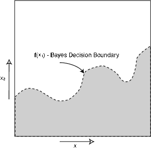
To connect these concepts to our classification scenario consider a simple example. Let $\eta \left(x\right)=P(Y=1|X=x)$ and assume $\eta \left(x\right)$ has the form

where $f:[0,1]\to [0,1]$ is Lipschitz with Lipschitz constant $L$ . The Bayes classifier is then given by

This is depicted in [link] . Note that this is a special, restricted class of problems. That is, we areconsidering the subset of all classification problems such that the joint distribution $P_{XY}$ satisfies $P(Y=1|X=x)=1/2+x_2-f\left(x_1\right)$ for some function $f$ that is Lipschitz. The Bayes decision boundary is therefore given by

Has we observed before this set has box-counting dimension 1.