| << Chapter < Page | Chapter >> Page > |
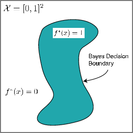
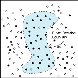
Given i.i.d. training pairs, , we want to construct a classifier that performs well on average, i.e., we want as close to as possible. In [link] (b) an example of the i.i.d. training pairs is depicted.
The construction of a classifier boils down to the estimation of the Bayes decision boundary. The histogram rule, discussed in aprevious lecture, approaches the problem by subdividing the feature space into small boxes and taking a majority vote of thetraining data in each box. A typical result is depicted in [link] (a).
The main problem with the histogram rule is that it is solving a more complicated problem than it is actually necessary. We do notneed to determine the correct label for each individual box directly (the histogram rule is essentially estimating ). In principle we only need to locate the decision boundary andassign the correct label on either side (notice that the accuracy of a majority vote over a region increases with the size of theregion). The next example illustrates this.
The pictures below correspond to the approximation of the Bayes classifier by three different classifiers:
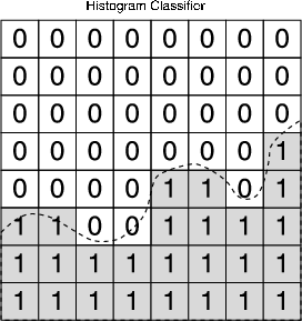
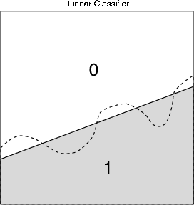
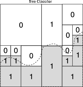
The linear classifier and the tree classifier (to be defined formally later) both attack the problem of finding the boundarymore directly than the histogram classifier, and therefore they tend to produce much better results in theory and practice. In thefollowing we will demonstrate this for classification trees.
Binary classification trees are constructed by a two-step process:
The basic idea is to first grow a very large, complicated tree classifier, that explains the the training data very accurately,but has poor generalization characteristics, and then prune this tree, to avoid overfitting.
The growing process is based on recursively subudividing the feature space. Usually the subdivisions are splits of existingregions into two smaller regions ( i.e., binary splits) and usually the splits are perpendicular to one of the feature axes. Anexample of such construction is depicted in [link] .

Often the splitting process is based on the training data, and is designed to separate data with different labels as much as possible.It such constructions, the “splits,” and hence the tree-structure itself, are data dependent. Alternatively, the splitting andsubdivision could be independent from the training data. The latter approach is the one we are going to investigate in detail, and we willconsider Dyadic Decision Trees and Recursive Dyadic Partitions (depicted in [link] ) in particular.
Until now we have been referring to trees, but did not make clear how do trees relate to partitions. It turns out that any decision tree canbe associated with a partition of the input space and vice-versa. In particular, a Recursive Dyadic Partition (RDP) can beassociated with a (binary) tree. In fact, this is the most efficient way of describing a RDP. In [link] we illustrate theprocedure. Each leaf of the tree corresponds to a cell of the partition. The nodes in the tree correspond to the various partitioncells that are generated through in the construction of the tree. The orientation of the dyadic split alternates between the levels of thetree (for the example of [link] , at the root level the split is done in the horizontal axis, at the level below that (thelevel of nodes 2 and 3) the split is done in the vertical axis, and so on...). The tree is called dyadic because the splits of cells are alwaysat the midpoint along one coordinate axis, and consequently the sidelengths of all cells are dyadic (i.e., powers of 2).

Notification Switch
Would you like to follow the 'Statistical learning theory' conversation and receive update notifications?