| << Chapter < Page | Chapter >> Page > |
Once the data has been collected, it must be organised in a manner that allows for the information to be extracted most efficiently. One method of organisation is to display the data in the form of graphs. Functions and graphs have been studied in Functions and Graphs , and similar techniques will be used here. However, instead of drawing graphs from equations as was done in Functions and graphs , bar graphs, histograms and pie charts will be drawn directly from the data.
A bar chart is used to present data where each observation falls into a specific category and where the categories, this is often for qualitative data. The frequencies (or percentages) are listed along the -axis and the categories are listed along the -axis. The heights of the bars correspond to the frequencies. The bars are of equal width and should not touch neighbouring bars.
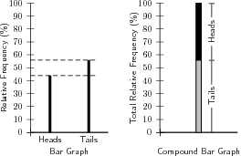
A compound bar chart (also called component bar chart) is a variant: here the bars are cut into various components depending on what is being shown. If percentages are used for various components of a compound bar, then the total bar height must be 100%. The compound bar chart is a little more complex but if this method is used sensibly, a lot of information can be quickly shown in an attractive fashion.
Examples of a bar and a compound bar graph, for Data Set 1 , are shown in [link] . According to the frequency table for Data Set 1, the coin landed heads-up 44 times and tails-up 56 times.

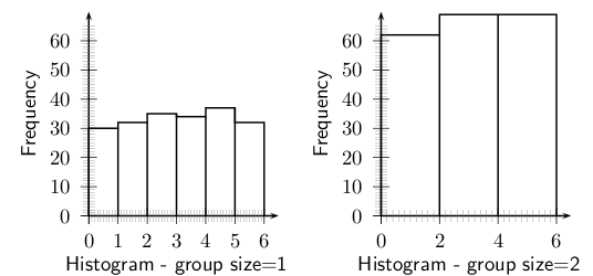
It is often useful to look at the frequency with which certain values fall in pre-set groups or classes of specified sizes. The choice of the groups should be such that they help highlight features in the data. If these grouped values are plotted in a manner similar to a bar graph, then the resulting graph is known as a histogram. Examples of histograms are shown in [link] for Data Set 2, with group sizes of 1 and 2.
| Groups | 1 | 2 | 3 | 4 | 5 | 6 |
| Frequency | 30 | 32 | 35 | 34 | 37 | 32 |
| Groups | 2 | 4 | 6 |
| Frequency | 62 | 69 | 69 |

The same data used to plot a histogram are used to plot a frequency polygon, except the pair of data values are plotted as a point and the points are joined with straight lines. The frequency polygons for the histograms in [link] are shown in [link] .


Notification Switch
Would you like to follow the 'Siyavula textbooks: grade 10 maths [ncs]' conversation and receive update notifications?