| << Chapter < Page | Chapter >> Page > |
The mixed-radix approach utilizes clever subsampling of and permutations of twiddle factor matrices to lower operation counts. The first step is to compute the prime factorization of the signal length . Prime factors of 2 and 3 are then combined to create as many factors of 4 and 6 as possible. The resulting prime factorization has the form . We can then perform a single step of the algorithm by computing FFTs of length .
Four unique matrix constructions are necessary to generalize a single step of the algorithm. The first is the identity matrix . The second is the permutation matrix , where
Note that swaps positions and in a vector. The third matrix to consider is a diagonal matrix of twiddle factors , where
with . The fourth and final matrix construction to consider is the standard DFT matrix .
The mixed-radix algorithm requires the interaction of operations on the subspaces , and so it is necessary to consider the Kronecker Product in calculations. The Kronecker Product is an operation defined as . If , then
Using these matrices, it possible to compose a single steps using the following equation [link] :
where
Note that .
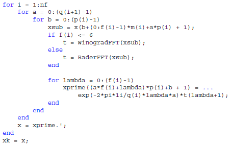
To implement the algorithm, each stage is applied iteratively to acquire . may be simplified into two separate steps using the definitions of each matrix to yield the following algorithm structure:

The DFT module in the above code utilizes the Winograd Short-Length Transforms to minimize operations when computing DFTs of length less than 6. For all other lengths, Rader's FFT is used.
Rader's FFT for prime lengths exploits results from number theory to express the DFT as a composite-length cyclic convolution [link] . Any prime number defines a multiplicative group modulo , denoted . This group is cyclic, i.e., , where is known as the primitive root modulo and . In practice, there is no general formula for finding for , but in this implementation is known and therefore may be stored in a lookup table.
The general form of the DFT of length is given by
Since the twiddle factor, , is naturally computed modulo and both and range from , we can rewrite the above formula using :
This formulation is of the form of a cyclic convolution of two sequences and where and of length . This convolution is computed via the convolution theorem:
For speed, the sequence is zero-padded between its zeroth and first index to a length which is a power of 2 such that and is cyclically repeated to be length . Since is known, it is possible to store the DFT of the sequence in a lookup table. The DFT of is then computed using the standard radix-2 Cooley-Tukey algorithm. The two DFTs are multiplied pointwise and then the inverse DFT is again calculated using the standard Cooley-Tukey algorithm. The first elements are then the result of the cyclic convolution. The final result is attained after adding back the DC offset.
For small numerical examples demonstrating this implementation of Rader's FFT, see this excellent guide here .

Notification Switch
Would you like to follow the 'Elec 301 projects fall 2014' conversation and receive update notifications?