| << Chapter < Page | Chapter >> Page > |
In some data sets, there are values (observed data points) called outliers . Outliers are observed data points that are far from the least squares line. They have large "errors", where the "error" or residual is the vertical distance from the line to the point.
Outliers need to be examined closely. Sometimes, for some reason or another, they should not be included in the analysis ofthe data. It is possible that an outlier is a result of erroneous data. Other times, an outlier may hold valuable information about the population under study and should remain included in the data. The key is to carefully examinewhat causes a data point to be an outlier.
Besides outliers, a sample may contain one or a few points that are called influential points . Influential points are observed data points that are far from the other observed data points in the horizontal direction. These points may have a big effect on the slope of the regression line. To begin to identify an influential point, you can remove it from the data set and see if the slope of the regression line is changed significantly.
Computers and many calculators can be used to identify outliers from the data. Computer output for regression analysis will often identify both outliers and influential points so that you can examine them.
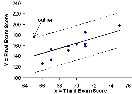
We can do this visually in the scatterplot by drawing an extra pair of lines that are two standard deviations above and below the best fit line. Any data points that are outside this extra pair of lines are flagged as potential outliers. Or we can do this numerically by calculating each residual and comparing it to twice the standard deviation. On the TI-83, 83+, or 84+, the graphical approach is easier. The graphical procedure is shown first, followed by the numerical calculations. You would generally only need to use one of these methods.
In the third exam/final exam example , you can determine if there is an outlier or not. If there is an outlier, as an exercise, delete it and fit the remaining data to a new line. For thisexample, the new line ought to fit the remaining data better. This means the SSE should be smaller and the correlation coefficient ought to be closer to 1 or -1.
As we did with the equation of the regression line and the correlation coefficient, we will use technology to calculate this standard deviation for us. Using the LinRegTTest with this data, scroll down through the output screens to find s=16.412
Line Y2=-173.5+4.83
-2(16.4) and line Y3=-173.5+4.83
+2(16.4)
where
=-173.5+4.83x is the line of best fit. Y2 and Y3 have the same slope as the line of best fit.
Graph the scatterplot with the best fit line in equation Y1, then enter the two extra lines as Y2 and Y3 in the "Y="equation editor and press ZOOM 9. You will find that the only data point that is not between lines Y2 and Y3 is the point x=65, y=175. On the calculator screen it is just barely outside these lines. The outlier is the student who had a grade of 65 on the third exam and 175 on the final exam; this point is further than 2 standard deviations away from the best fit line.
Sometimes a point is so close to the lines used to flag outliers on the graph that it is difficult to tell if the point is between or outside the lines. On a computer, enlarging the graph may help; on a small calculator screen, zooming in may make the graph clearer. Note that when the graph does not give a clear enough picture, you can use the numerical comparisons to identify outliers.

is the standard deviation of all the values where = the total number of data points. If each residual is calculated and squared, and the results are added, we get the SSE. The standard deviation of the residuals is calculated from the SSE as:
Rather than calculate the value of ourselves, we can find using the computer or calculator. For this example, the calculator function LinRegTTest found as the standard deviation of the residuals
| 65 | 175 | 140 | |
| 67 | 133 | 150 | |
| 71 | 185 | 169 | |
| 71 | 163 | 169 | |
| 66 | 126 | 145 | |
| 75 | 198 | 189 | |
| 67 | 153 | 150 | |
| 70 | 163 | 164 | |
| 71 | 159 | 169 | |
| 69 | 151 | 160 | |
| 69 | 159 | 160 |
We are looking for all data points for which the residual is greater than =2(16.4)=32.8 or less than -32.8. Compare these values to the residuals in column 4 of the table. The only such data point is the student who had a grade of 65 on the third exam and 175 on the final exam; the residual for this student is 35.
and
The new line with is a stronger correlation than the original ( =0.6631) because is closer to 1. This means that the new line is a better fit to the 10 remaining data values. The line can better predict the final exam score given the third exam score.

Notification Switch
Would you like to follow the 'Elementary statistics' conversation and receive update notifications?