3.2 Graphical analysis of one-dimensional motion  (Page 9/8)

A graph, like a picture, is worth a thousand words. Graphs not only contain numerical information; they also reveal relationships between physical quantities. This section uses graphs of displacement, velocity, and acceleration versus time to illustrate one-dimensional kinematics.

Slopes and general relationships

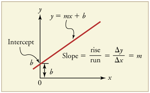
First note that graphs in this text have perpendicular axes, one horizontal and the other vertical. When two physical quantities are plotted against one another in such a graph, the horizontal axis is usually considered to be an independent variable    and the vertical axis a dependent variable    . If we call the horizontal axis the $x$ -axis and the vertical axis the $y$ -axis, as in [link] , a straight-line graph has the general form

Here $m$ is the slope    , defined to be the rise divided by the run (as seen in the figure) of the straight line. The letter $b$ is used for the y -intercept , which is the point at which the line crosses the vertical axis.

Graph of displacement vs. time ( a = 0, so v Is constant)

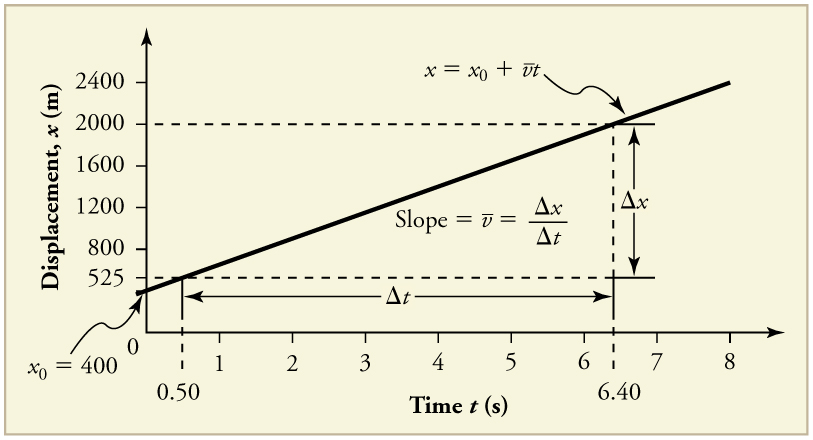
Time is usually an independent variable that other quantities, such as displacement, depend upon. A graph of displacement versus time would, thus, have $x$ on the vertical axis and $t$ on the horizontal axis. [link] is just such a straight-line graph. It shows a graph of displacement versus time for a jet-powered car on a very flat dry lake bed in Nevada.

Using the relationship between dependent and independent variables, we see that the slope in the graph above is average velocity $\stackrel{-}{v}$ and the intercept is displacement at time zero—that is, $x_0$ . Substituting these symbols into $y=\text{mx}+b$ gives

or

Thus a graph of displacement versus time gives a general relationship among displacement, velocity, and time, as well as giving detailed numerical information about a specific situation.

From the figure we can see that the car has a displacement of 25 m at 0.50 s and 2000 m at 6.40 s. Its displacement at other times can be read from the graph; furthermore, information about its velocity and acceleration can also be obtained from the graph.