| << Chapter < Page | Chapter >> Page > |
Before filtering, we take the lists of spectral peaks that is the output of the landmarks generator algorithm and generate matrices that are the same size as the spectrograms, with the peaks replaced by 1’s in their respective positions and all other points replaced by 0’s. At some point during our project we had the idea of convolving this matrix with a Gaussian curve, in order to allow peaks to match somewhat if they were shifted only slightly. However, we later determined that even a very small Gaussian would worsen our noise resistance, so this idea was dropped. So basically now we have one map for each song that shows the position in time and frequency bins of all peaks. Next we normalize these matrices using their Frobenius norm. This ensures that the final score is normalized. Then we apply the matched filter which basically consists of flipping one of the matrices and convolving them, which is done by zero padding them both to the proper size and multiplying their 2D FFT’s, for speed. The result is a cross correlation matrix, but we still need to extract a single number from it to be our match score.
Through much testing, we determined that the most accurate and noise-resistant measure of the match was simply taking the global maximum of the result. Other approaches that we tried, such as taking the trace of the X T X or the sum of the global maxima for each row or column, had much more frequent mismatches. Taking just the global maximum of the whole matrix was simple and extremely effective.
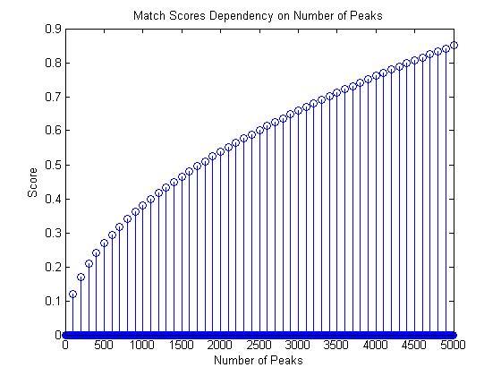
When looking at test results, however, we saw that the score still had a certain dependency on the size of the segments being compared. Through more testing, we determined that this dependency looked approximately like a dependency on the square root of the ratio of the lower number of peaks by the higher number of peaks, when testing with a noiseless fragment of a larger song. This can be seen in this plot:

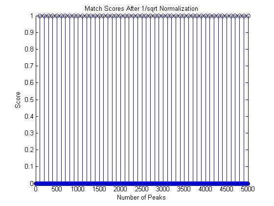
In the plot above, the original segment has 6915 peaks and the fragment was tested with between 100 and 5000 peaks, in intervals of 100. Since smaller sample sizes usually lead to having fewer peaks, we had to get rid of this dependency. To prevent the square root growth of the scores, the final score is multiplied by the inverse of this square root, yielding a match score that is approximately independent of sample size. This can be seen in the next stem plot, made with the same segments as the first:

So clearly this allows us to get better match scores with small song segments. After this process, we had a score that was approximately independent of segment size, normalized and could tell apart matches and mismatches, even with lots of noise. All that was left was to test it against different sets of data and set a threshold for distinguishing between matches and non-matches.
The filter’s behavior proved to be very consistent. Perfect matches (trying to match a segment with itself) always got scores of 1. Matching noiseless segments to the whole song usually yielded scores in the upper .8’s or in the .9’s, with a few rare exceptions that could have been caused by a bad choice of segment, such as a segment with a long period of silence, for example. Noisy segments usually gave us low scores such as in the .1’s, but more importantly mismatches were even lower, in the .05’s to .07’s or so. This allowed us to set a threshold for determining when we have a match or not.
During our testing, we considered using a statistical approach to set the threshold. For example, if we wanted a 95% certainty that a song matched, we could require the highest match score to be greater than 1.66*[σ/sqrt(n)] + µ, where σ is the standard deviation, n is the sample size and µ is the mean. However, with our very small sample size, this threshold seemed to yield inaccurate results, so the simple threshold criterion of the highest match having to be at least 1.5 times the second highest in order to be considered a match was used.
Even though we followed the ideas in the paper by Wang, we still had some significant differences from the approach used by Shazam. We followed the ideas they had for fingerprint creation, to a certain extent, however the company uses hash tables instead of matched filters to perform the comparison. While evidently faster than using a matched filter, hash tables are not covered in ELEC 301. Furthermore, when making a hash, Wang says they combine several points in an area with an anchor point and pair them up combinatorially. This allows the identification of a time offset to be used with the hash tables and makes the algorithm even faster and more robust. Perhaps investigating this would be an interesting extension of the project, if we had more time.

Notification Switch
Would you like to follow the 'Digital song analysis using frequency analysis' conversation and receive update notifications?