0.16 Markov chains  (Page 4/4)

Three companies, $A$ , $B$ , and $C$ , compete against each other. The transition matrix T for people switching each month among them is given by the following transition matrix.

If the initial market share for the companies $A$ , $B$ , and $C$ is $\left[\begin{array}{ccc}\text{.}\text{25}& \text{.}\text{35}& \text{.}\text{40}\end{array}\right]$ , what is the long term distribution?

Since the long term market share does not depend on the initial market share, we can simply raise the transition market share to a large power and get the distribution.

$T^{\text{20}}=\left[\begin{array}{ccc}\text{13}/\text{55}& 3/\text{11}& \text{27}/\text{55}\end{array}\right]$

Got questions? Get instant answers now!

Got questions? Get instant answers now!

We summarize as follows:

Regular markov chains

1. As we take higher powers of $T$ , $T^n$ , as n becomes large, approaches a state of equilibrium.
2. If $M$ is any distribution vector, and $E$ an equilibrium vector, then ${\text{MT}}^n=E$ .
3. Each row of the equilibrium matrix $T^n$ is a unique equilibrium vector $E$ such that $\text{ET}=E$ .
4. The equilibrium distribution vector $E$ can be found by letting $\text{ET}=E$ .

Absorbing markov chains

In this section, we will study a type of Markov chain in which when a certain state is reached, it is impossible to leave that state. Such states are called absorbing states , and a Markov Chain that has at least one such state is called an Absorbing Markov chain . Suppose you have the following transition matrix.

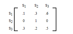
The state $S_2$ is an absorbing state, because the probability of moving from state $S_2$ to state $S_2$ is 1. Which is another way of saying that if you are in state $S_2$ , you will remain in state $S_2$ .

In fact, this is the way to identify an absorbing state. If the probability in row i and column i , $p_{\text{ii}}$ , is 1, then state $S_i$ is an absorbing state.

We begin with an application of absorbing Markov chains to the gambler's ruin problem.

Gambler's ruin problem

A gambler has $3,000, and she decides to gamble $1,000 at a time at a Black Jack table in a casino in Las Vegas. She has told herself that she will continue playing until she goes broke or has $5,000. Her probability of winning at Black Jack is $\text{.}\text{40}$ . Write the transition matrix, identify the absorbing states, find the solution matrix, and determine the probability that the gambler will be financially ruined at a stage when she has $2,000.

The transition matrix is written below. Clearly the state 0 and state $\mathrm{5K}$ are the absorbing states. This makes sense because as soon as the gambler reaches 0, she is financially ruined and the game is over. Similarly, if the gambler reaches $5,000, she has promised herself to quit and, again, the game is over. The reader should note that $p_{\text{00}}=1$ , and $p_{\text{55}}=1$ .

Further observe that since the gambler bets only $1,000 at a time, she can raise or lower her money only by $1,000 at a time. In other words, if she has $2,000 now, after the next bet she can have $3,000 with a probability of $\text{.}\text{40}$ and $1,000 with a probability of $\text{.}\text{60}$ .

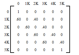
To determine the long term trend, we raise the matrix to higher powers until all the non- absorbing states are absorbed. This is the called the solution matrix .

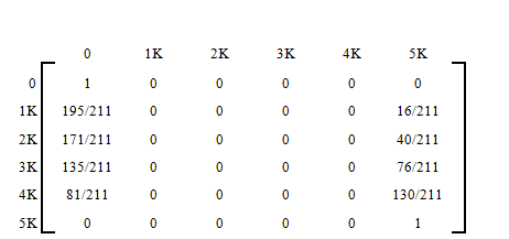
The solution matrix is often written in the following form, where the non-absorbing states are written as rows on the side, and the absorbing states as columns on the top.

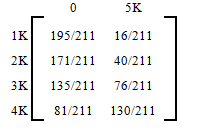
The table lists the probabilities of getting absorbed in state 0 or state 5K starting from any of the four non-absorbing states. For example, if at any instance the gambler has $3,000, then her probability of financial ruin is 135/211.

Got questions? Get instant answers now!

Got questions? Get instant answers now!

Solve the Gambler's Ruin Problem of [link] without raising the matrix to higher powers, and determine the number of bets the gambler makes before the game is over.

In solving absorbing states, it is often convenient to rearrange the matrix so that the rows and columns corresponding to the absorbing states are listed first. This is called the Canonical form . The transition matrix of [link] in the canonical form is listed below.

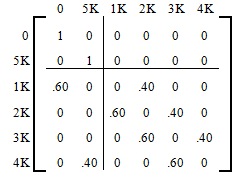
The canonical form divides the transition matrix into four sub-matrices as listed below.

The matrix $F={\left(1_n-B\right)}^{-1}$ is called the fundamental matrix for the absorbing Markov chain, where $I_n$ is an identity matrix of the same size as $B$ . The $i$ , $j-\text{th}$ entry of this matrix tells us the average number of times the process is in the non-absorbing state $j$ before absorption if it started in the non-absorbing state $i$ . The matrix $F$ for our problem is listed below.

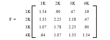
The Fundamental matrix $F$ helps us determine the average number of games played before absorption.

According to the matrix, the entry 1.78 in the row 3, column 2 position says that the gambler will play the game 1.78 times before she goes from $3K to $2K. The entry 2.25 in row 3, column 3 says that if the gambler now has $3K, she will have $3K on the average 2.25 times before the game is over.

We now address the question of how many bets will she have to make before she is absorbed, if the gambler begins with $3K?

If we add the number of games the gambler plays in each non-absorbing state, we get the average number of games before absorption from that state. Therefore, if the gambler starts with $3K, the average number of Black Jack games she will play before absorption is

$1\text{.}\text{07}+1\text{.}\text{78}+2\text{.}\text{25}+\text{.}\text{90}=6\text{.}0$

That is, we expect the gambler will either have $5,000 or nothing on the 7th bet.

Lastly, we find the solution matrix without raising the transition matrix to higher powers.

The matrix $\text{FA}$ gives us the solution matrix.

$\text{FA}=\left[\begin{array}{cccc}1\text{.}\text{54}& \text{.}\text{90}& \text{.}\text{47}& \text{.}\text{19}\\ 1\text{.}\text{35}& 2\text{.}\text{25}& 1\text{.}\text{18}& \text{.}\text{47}\\ 1\text{.}\text{07}& 1\text{.}\text{78}& 2\text{.}\text{25}& \text{.}\text{90}\\ \text{.}\text{64}& 1\text{.}\text{07}& 1\text{.}\text{35}& 1\text{.}\text{54}\end{array}\right]\left[\begin{array}{cc}\text{.}6& 0\\ 0& 0\\ 0& 0\\ 0& \text{.}4\end{array}\right]=\left[\begin{array}{cc}\text{.}\text{92}& \text{.}\text{08}\\ \text{.}\text{81}& \text{.}\text{19}\\ \text{.}\text{64}& \text{.}\text{36}\\ \text{.}\text{38}& \text{.}\text{62}\end{array}\right]$

Which is the same as the following matrix we obtained by raising the transition matrix to higher powers.

Got questions? Get instant answers now!

We summarize as follows:

Absorbing markov chains

1. A Markov chain is an absorbing Markov chain if it has at least one absorbing state. A state $i$ is an absorbing state if once the system reaches state $i$ , it stays in that state; that is, $p_{\text{ii}}=1$ .
2. If a transition matrix $T$ for an absorbing Markov chain is raised to higher powers, it reaches an absorbing state called the solution matrix and stays there. The $i$ , $j-\text{th}$ entry of this matrix gives the probability of absorption in state $j$ while starting in state $i$ .
3. Alternately, the solution matrix can be found in the following manner.
   1. Express the transition matrix in the canonical form as below.
      $T=\left[\begin{array}{cc}{I}_n& 0\\ A& B\end{array}\right]$
      
      where $I_n$ is an identity matrix, and 0 is a matrix of all zeros.
   2. The fundamental matrix $F={\left(I-B\right)}^{-1}$ . The fundamental matrix helps us find the number of games played before absorption.
   3. $\text{FA}$ is the solution matrix, whose $i$ , $j-\text{th}$ entry gives the probability of absorption in state $j$ while starting in state $i$ .
4. The sum of the entries of a row of the fundamental matrix gives us the expected number of steps before absorption for the non-absorbing state associated with that row.