| << Chapter < Page | Chapter >> Page > |
By the end of this section, you will be able to:
Controversy sometimes surrounds the prices and quantities established by demand and supply, especially for products that are considered necessities. In some cases, discontent over prices turns into public pressure on politicians, who may then pass legislation to prevent a certain price from climbing “too high” or falling “too low.”
The demand and supply model shows how people and firms will react to the incentives provided by these laws to control prices, in ways that will often lead to undesirable consequences. Alternative policy tools can often achieve the desired goals of price control laws, while avoiding at least some of their costs and tradeoffs.
Laws that government enacts to regulate prices are called Price controls . Price controls come in two flavors. A price ceiling keeps a price from rising above a certain level (the “ceiling”), while a price floor keeps a price from falling below a certain level (the “floor”). This section uses the demand and supply framework to analyze price ceilings. The next section discusses price floors.
In many markets for goods and services, demanders outnumber suppliers. Consumers, who are also potential voters, sometimes unite behind a political proposal to hold down a certain price. In some cities, such as Albany, renters have pressed political leaders to pass rent control laws, a price ceiling that usually works by stating that rents can be raised by only a certain maximum percentage each year.
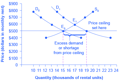
Rent control becomes a politically hot topic when rents begin to rise rapidly. Everyone needs an affordable place to live. Perhaps a change in tastes makes a certain suburb or town a more popular place to live. Perhaps locally-based businesses expand, bringing higher incomes and more people into the area. Changes of this sort can cause a change in the demand for rental housing, as [link] illustrates. The original equilibrium (E 0 ) lies at the intersection of supply curve S 0 and demand curve D 0 , corresponding to an equilibrium price of $500 and an equilibrium quantity of 15,000 units of rental housing. The effect of greater income or a change in tastes is to shift the demand curve for rental housing to the right, as shown by the data in [link] and the shift from D 0 to D 1 on the graph. In this market, at the new equilibrium E 1 , the price of a rental unit would rise to $600 and the equilibrium quantity would increase to 17,000 units.

| Price | Original Quantity Supplied | Original Quantity Demanded | New Quantity Demanded |
|---|---|---|---|
| $400 | 12,000 | 18,000 | 23,000 |
| $500 | 15,000 | 15,000 | 19,000 |
| $600 | 17,000 | 13,000 | 17,000 |
| $700 | 19,000 | 11,000 | 15,000 |
| $800 | 20,000 | 10,000 | 14,000 |

Notification Switch
Would you like to follow the 'Principles of macroeconomics for ap® courses' conversation and receive update notifications?