| << Chapter < Page | Chapter >> Page > |
The following examples illustrate a left-, right-, and two-tailed test.
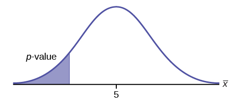
H o : μ = 5, H a : μ <5
Test of a single population mean. H a tells you the test is left-tailed. The picture of the p -value is as follows:
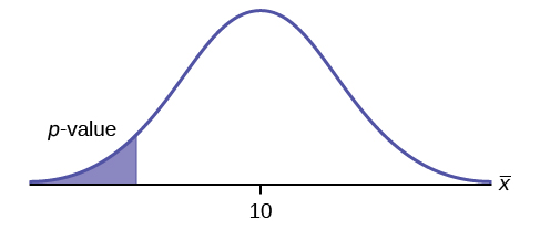
H 0 : μ = 10, H a : μ <10
Assume the p -value is 0.0935. What type of test is this? Draw the picture of the p -value.
left-tailed test
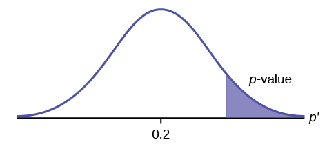
H 0 : p ≤ 0.2 H a : p >0.2
This is a test of a single population proportion. H a tells you the test is right-tailed . The picture of the p -value is as follows:
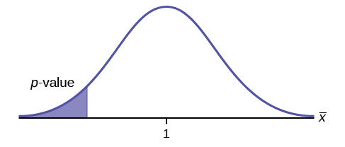
H 0 : μ ≤ 1, H a : μ >1
Assume the p -value is 0.1243. What type of test is this? Draw the picture of the p -value.
right-tailed test
H 0 : p = 50 H a : p ≠ 50
This is a test of a single population mean. H a tells you the test is two-tailed . The picture of the p -value is as follows.
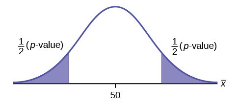
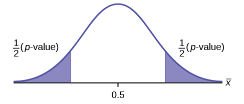
H 0 : p = 0.5, H a : p ≠ 0.5
Assume the p -value is 0.2564. What type of test is this? Draw the picture of the p -value.
two-tailed test
Jeffrey, as an eight-year old, established a mean time of 16.43 seconds for swimming the 25-yard freestyle, with a standard deviation of 0.8 seconds . His dad, Frank, thought that Jeffrey could swim the 25-yard freestyle faster using goggles. Frank bought Jeffrey a new pair of expensive goggles and timed Jeffrey for 15 25-yard freestyle swims . For the 15 swims, Jeffrey's mean time was 16 seconds. Frank thought that the goggles helped Jeffrey to swim faster than the 16.43 seconds. Conduct a hypothesis test using a preset α = 0.05. Assume that the swim times for the 25-yard freestyle are normal.
Set up the Hypothesis Test:
Since the problem is about a mean, this is a test of a single population mean .
H 0 : μ = 16.43 H a : μ <16.43
For Jeffrey to swim faster, his time will be less than 16.43 seconds. The "<" tells you this is left-tailed.
Determine the distribution needed:
Random variable: = the mean time to swim the 25-yard freestyle.
Distribution for the test: is normal (population standard deviation is known: σ = 0.8)
Therefore,
μ = 16.43 comes from H 0 and not the data. σ = 0.8, and n = 15.
Calculate the p -value using the normal distribution for a mean:
p -value = P ( <16) = 0.0187 where the sample mean in the problem is given as 16.
p -value = 0.0187 (This is called the actual level of significance .) The p -value is the area to the left of the sample mean is given as 16.
Graph:
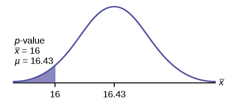
μ = 16.43 comes from H 0 . Our assumption is μ = 16.43.
Interpretation of the p -value: If H 0 is true , there is a 0.0187 probability (1.87%)that Jeffrey's mean time to swim the 25-yard freestyle is 16 seconds or less. Because a 1.87% chance is small, the mean time of 16 seconds or less is unlikely to have happened randomly. It is a rare event.
Compare α and the p -value:
α = 0.05 p -value = 0.0187 α > p -value
Make a decision: Since α > p -value, reject H 0 .
This means that you reject μ = 16.43. In other words, you do not think Jeffrey swims the 25-yard freestyle in 16.43 seconds but faster with the new goggles.
Conclusion: At the 5% significance level, we conclude that Jeffrey swims faster using the new goggles. The sample data show there is sufficient evidence that Jeffrey's mean time to swim the 25-yard freestyle is less than 16.43 seconds.
The p -value can easily be calculated.
Press
STAT and arrow over to
TESTS . Press
1:Z-Test . Arrow over to
Stats and press
ENTER . Arrow down and enter 16.43 for
μ
0 (null hypothesis), .8 for
σ , 16 for the sample mean, and 15 for
n . Arrow down to
μ : (alternate hypothesis) and arrow over to<
μ
0 . Press
ENTER . Arrow down to
Calculate and press
ENTER . The calculator not only calculates the
p -value (
p = 0.0187) but it also calculates the test statistic (
z -score) for the sample mean.
μ <16.43 is the alternative hypothesis. Do this set of instructions again except arrow to
Draw (instead of
Calculate ). Press
ENTER . A shaded graph appears with
z = -2.08 (test statistic) and
p = 0.0187 (
p -value). Make sure when you use
Draw that no other equations are highlighted in
Y = and the plots are turned off.
When the calculator does a
Z -Test, the
Z-Test function finds the
p -value by doing a normal probability calculation using the
central limit theorem :
2nd DISTR normcdf
.
The Type I and Type II errors for this problem are as follows:
The Type I error is to conclude that Jeffrey swims the 25-yard freestyle, on average, in less than 16.43 seconds when, in fact, he actually swims the 25-yard freestyle, onaverage, in 16.43 seconds. (Reject the null hypothesis when the null hypothesis is true.)
The Type II error is that there is not evidence to conclude that Jeffrey swims the 25-yard free-style, on average, in less than 16.43 seconds when, in fact, he actually does swim the 25-yard free-style, on average, in less than 16.43 seconds. (Do not reject the null hypothesis when the null hypothesis is false.)

Notification Switch
Would you like to follow the 'Introductory statistics' conversation and receive update notifications?