2.4 Distribution of molecular speeds  (Page 31/9)

Particles in an ideal gas all travel at relatively high speeds, but they do not travel at the same speed. The rms speed is one kind of average, but many particles move faster and many move slower. The actual distribution of speeds has several interesting implications for other areas of physics, as we will see in later chapters.

The maxwell-boltzmann distribution

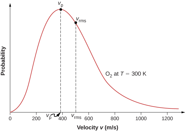
The motion of molecules in a gas is random in magnitude and direction for individual molecules, but a gas of many molecules has a predictable distribution of molecular speeds. This predictable distribution of molecular speeds is known as the Maxwell-Boltzmann distribution    , after its originators, who calculated it based on kinetic theory, and it has since been confirmed experimentally ( [link] ).

To understand this figure, we must define a distribution function of molecular speeds, since with a finite number of molecules, the probability that a molecule will have exactly a given speed is 0.

We define the distribution function $f(v)$ by saying that the expected number $N(v_1,v_2)$ of particles with speeds between $v_1$ and $v_2$ is given by

[Since N is dimensionless, the unit of f ( v ) is seconds per meter.] We can write this equation conveniently in differential form:

In this form, we can understand the equation as saying that the number of molecules with speeds between v and $v+dv$ is the total number of molecules in the sample times f ( v ) times dv . That is, the probability that a molecule’s speed is between v and $v+dv$ is f ( v ) dv .

We can now quote Maxwell’s result, although the proof is beyond our scope.

The factors before the $v^2$ are a normalization constant; they make sure that $N(0,\infty )=N$ by making sure that ${\displaystyle {\int }_0^{\infty }f(v)dv=1}.$ Let’s focus on the dependence on v . The factor of $v^2$ means that $f(0)=0$ and for small v , the curve looks like a parabola. The factor of $e^{\text{−}{m}_0{v}^2\text{/}2k_{\text{B}}T}$ means that $\underset{v\to \infty }{\text{lim}}f(v)=0$ and the graph has an exponential tail, which indicates that a few molecules may move at several times the rms speed. The interaction of these factors gives the function the single-peaked shape shown in the figure.