| << Chapter < Page | Chapter >> Page > |
In Grade 11 you were introduced to linear programming and solved problems by looking at points on the edges of the feasible region. In Grade 12 you will look at how to solve linear programming problems in a more general manner.
Here is a recap of some of the important concepts in linear programming.
Constraints mean that we cannot just take any and when looking for the and that optimise our objective function. If we think of the variables and as a point in the -plane then we call the set of all points in the -plane that satisfy our constraints the feasible region . Any point in the feasible region is called a feasible point .
For example, the constraints
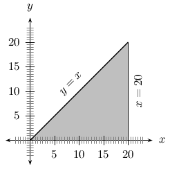
mean that every we can consider must lie in the first quadrant of the plane. The constraint
means that every must lie on or below the line and the constraint
means that must lie on or to the left of the line .
We can use these constraints to draw the feasible region as shown by the shaded region in [link] .

| If , feasible points must lie on the line | |
| If , feasible points must lie on the line | |
| If , feasible points must lie on or below the line . | |
| If , feasible points must lie on or to the left of the line . |
When a constraint is linear, it means that it requires that any feasible point lies on one side of or on a line. Interpreting constraints as graphs in the plane is very important since it allows us to construct the feasible region such as in [link] .
If the objective function and all of the constraints are linear then we call the problem of optimising the objective function subject to these constraints a linear program . All optimisation problems we will look at will be linear programs.
The major consequence of the constraints being linear is that the feasible region is always a polygon. This is evident since the constraints that define the feasible region all contribute a line segment to its boundary (see [link] ). It is also always true that the feasible region is a convex polygon.
The objective function being linear means that the feasible point(s) that gives the solution of a linear program always lies on one of the vertices of the feasible region . This is very important since, as we will soon see, it gives us a way of solving linear programs.
We will now see why the solutions of a linear program always lie on the vertices of the feasible region. Firstly, note that if we think of as lying on the axis, then the function (where and are real numbers) is the definition of a plane. If we solve for in the equation defining the objective function then
What this means is that if we find all the points where for any real number (i.e. is constant with a value of ), then we have the equation of a line. This line we call a level line of the objective function.

Notification Switch
Would you like to follow the 'Siyavula textbooks: grade 12 maths' conversation and receive update notifications?