9.4 Matched or paired samples

Quantitative information analysis Page 1 / 1

This module provides an overview of Hypothesis Testing: Matched or Paired Samples as a part of Collaborative Statistics collection (col10522) by Barbara Illowsky and Susan Dean.

Simple random sampling is used.
Sample sizes are often small.
Two measurements (samples) are drawn from the same pair of individuals or objects.
Differences are calculated from the matched or paired samples.
The differences form the sample that is used for the hypothesis test.
The matched pairs have differences that either come from a population that is normal or the number of differences is sufficiently large so the distribution of the sample mean of differences is approximately normal.

In a hypothesis test for matched or paired samples, subjects are matched in pairs and differences are calculated. The differences are the data. Thepopulation mean for the differences, $μ_{d}$ , is then tested using a Student-t test for a single population mean with $n - 1$ degrees of freedom where $n$ is the number of differences.

The test statistic (t-score) is:

t = \frac{\bar{x_{d}} - μ_{d}}{(\frac{s_{d}}{\sqrt{n}})}

Matched or paired samples

A study was conducted to investigate the effectiveness of hypnotism in reducing pain. Results forrandomly selected subjects are shown in the table. The "before" value is matched to an "after" value and the differences are calculated. The differences have a normal distribution.

Subject:	A	B	C	D	E	F	G	H
Before	6.6	6.5	9.0	10.3	11.3	8.1	6.3	11.6
After	6.8	2.4	7.4	8.5	8.1	6.1	3.4	2.0

Are the sensory measurements, on average, lower after hypnotism? Test at a 5% significance level.

Corresponding "before" and "after" values form matched pairs. (Calculate "sfter" - "before").

After Data	Before Data	Difference
6.8	6.6	0.2
2.4	6.5	-4.1
7.4	9	-1.6
8.5	10.3	-1.8
8.1	11.3	-3.2
6.1	8.1	-2
3.4	6.3	-2.9
2	11.6	-9.6

The data for the test are the differences:{0.2, -4.1, -1.6, -1.8, -3.2, -2, -2.9, -9.6}

The sample mean and sample standard deviation of the differences are: $x_{d} = -3.13$ and $s_{d} = 2.91$ Verify these values.

Let $μ_{d}$ be the population mean for the differences. We use the subscript $d$ to denote "differences."

Random Variable: $X_{d}$ = the mean difference of the sensory measurements

H_{o} : μ_{d} \geq 0

There is no improvement. (

μ_{d}

is the population mean of the differences.)

H_{a} : μ_{d} < 0

There is improvement. The score should be lower after hypnotism so the difference ought to be negativeto indicate improvement.

Distribution for the test: The distribution is a student-t with $df = n - 1 = 8 - 1 = 7$ . Use $t_{7}$ . (Notice that the test is for a single population mean.)

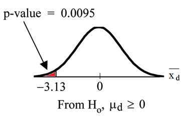
Calculate the p-value using the Student-t distribution: $p-value = 0.0095$

Graph:

Normal distribution curve of the average difference of sensory measurements with values of -3.13 and 0. A vertical upward line extends from -3.13 to the curve, and the p-value is indicated in the area to the left of this value.

$X_{d}$ is the random variable for thedifferences.

The sample mean and sample standarddeviation of the differences are:

$x_{d} = -3.13$

$s_{d} = 2.91$

Compare $α$ and the p-value: $α = 0.05$ and $p-value = 0.0095$ . $α > p-value$ .

Make a decision: Since $α > p-value$ , reject $H_{o}$ .

This means that $μ_{d} < 0$ and there is improvement.

Conclusion: At a 5% level of significance, from the sample data, there is sufficient evidence to conclude that the sensory measurements, on average, are lower afterhypnotism. Hypnotism appears to be effective in reducing pain.

For the TI-83+ and TI-84 calculators, you can either calculate the differences ahead of time ( after - before ) and put the differences into a list or you can put the after data into a first list and the before data into a second list. Then go to a third list and arrow up to the name. Enter 1st list name - 2nd list name. The calculatorwill do the subtraction and you will have the differences in the third list.

TI-83+ and TI-84: Use your list of differences as the data. Press STAT and arrow over to TESTS . Press 2:T-Test . Arrow over to Data and press ENTER . Arrow down and enter 0 for

μ_{0}

, the name of the list where you put the data, and 1 for Freq:. Arrow down to μ : and arrow over to <

μ_{0}

. Press ENTER . Arrow down to Calculate and press ENTER . The p-value is 0.0094 and the test statistic is -3.04. Do these instructions again exceptarrow to Draw (instead of Calculate ). Press ENTER .

A college football coach was interested in whether the college's strength development class increased his players' maximum lift (in pounds) on the benchpress exercise. He asked 4 of his players to participate in a study. The amount of weight they could each lift was recorded before they took the strength developmentclass. After completing the class, the amount of weight they could each lift was again measured. The data are as follows:

Weight (in pounds)	Player 1	Player 2	Player 3	Player 4
Amount of weighted lifted prior to the class	205	241	338	368
Amount of weight lifted after the class	295	252	330	360

The coach wants to know if the strength development class makes his players stronger, on average.

Record the differences data. Calculate the differences by subtracting the amount of weight lifted prior to the class from the weight lifted after completing the class. Thedata for the differences are: {90, 11, -8, -8}. The differences have a normal distribution.

Using the differences data, calculate the sample mean and the sample standard deviation.

$x_{d} = 21.3 s_{d} = 46.7$

Using the difference data, this becomes a test of a single __________ (fill in the blank).

Define the random variable: $X_{d} =$ mean difference in the maximum lift per player.

The distribution for the hypothesis test is $t_{3}$ .

$H_{o} : μ_{d} \leq 0 H_{a} : μ_{d} > 0$

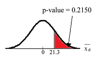
Graph:

Normal distribution curve with values of 0 and 21.3. A vertical upward line extends from 21.3 to the curve and the p-value is indicated in the area to the right of this value.

Calculate the p-value: The p-value is 0.2150

Decision: If the level of significance is 5%, the decision is to not reject the null hypothesis because $α < p-value$ .

What is the conclusion?

means; At a 5% level of significance, from the sample data, there is not sufficient evidence to conclude that the strength development class helped to make the players stronger, on average.

Seven eighth graders at Kennedy Middle School measured how farthey could push the shot-put with their dominant (writing) hand and their weaker (non-writing) hand. They thought that they could push equal distances with eitherhand. The following data was collected.

Distance (in feet) using	Student 1	Student 2	Student 3	Student 4	Student 5	Student 6	Student 7
Dominant Hand	30	26	34	17	19	26	20
Weaker Hand	28	14	27	18	17	26	16

Conduct a hypothesis test to determine whether the mean difference in distances between the children's dominant versus weaker hands is significant.

Hint use a t-test on the difference data. Assume the differences have a normal distribution. The random variable is the mean difference.

Check The test statistic is 2.18 and the p-value is 0.0716.

What is your conclusion?

$H_{0}$ : $μ_{d}$ equals 0; $H_{a}$ : $μ_{d}$ does not equal 0; Do not reject the null; At a 5% significance level, from the sample data, there is not sufficient evidence to conclude that the mean difference in distances between the children's dominant versus weaker hands is significant (there is not sufficient evidence to show that the children could push the shot-put further with their dominant hand). Alpha and the p-value are close so the test is not strong.

<< Chapter < Page Page > Chapter >>

Read also:

Get Jobilize Job Search Mobile App in your pocket Now!

100% Free Mobile Applications
Receive real-time job alerts and never miss the right job again

Source: OpenStax, Quantitative information analysis iii. OpenStax CNX. Dec 25, 2009 Download for free at http://cnx.org/content/col11155/1.1

Google Play and the Google Play logo are trademarks of Google Inc.

Notification Switch

Would you like to follow the 'Quantitative information analysis iii' conversation and receive update notifications?

Ask

	1 Pharmacology Nervous System MCQ By Rohini Ajay Start Quiz
©flickr: Gareth	Resume Writing MCQ By Abby Sharp Start Quiz
©flickr: Dutch	Las Vegas Timeshare By Donyea Sweets Start Test
	Chemistry Final By Briana Hamilton Start Flashcards
©flickr:	Morphology By Jugnu Khan Start Quiz
©flickr: U.S.	Biology Chapter 9 By Michael Sag Start Exam
	1 AP Key Terms 01 Human Body Anatomy Physiology By OpenStax Start Key Terms
	9 Arts Society: Theater 9 Exam By Jonathan Long Start Exam
	13 Dr Garry GI Ruminants quiz By Brooke Delaney Start Exam
	4 Gang of Four Design Patterns By JavaChamp Team Start Quiz