| << Chapter < Page | Chapter >> Page > |
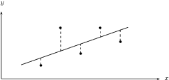
We now come to a more accurate method of finding the line of best-fit. The method is very simple. Suppose we guess a line of best-fit. Then at at every data point, we find the distance between the data point and the line. If the line fitted the data perfectly, this distance should be zero for all the data points. The worse the fit, the larger the differences. We then square each of these distances, and add them all together.

The best-fit line is then the line that minimises the sum of the squared distances.
Suppose we have a data set of points . We also have a line that we are trying to fit to the data. The distance between the first data point and the line, for example, is
We now square each of these distances and add them together. Lets call this sum . Then we have that
Thus our problem is to find the value of and such that is minimised. Let us call these minimising values and . Then the line of best-fit is . We can find and using calculus, but it is tricky, and we will just give you the result, which is that
Khan academy video on regression - 1
In the table below, we have the records of the maintenance costs in Rands, compared with the age of the appliance in months. We have data for 5 appliances.
| appliance | 1 | 2 | 3 | 4 | 5 |
| age ( ) | 5 | 10 | 15 | 20 | 30 |
| cost ( ) | 90 | 140 | 250 | 300 | 380 |
Find the line of best fit using the method of least squares.
| appliance | ||||
| 1 | 5 | 90 | 450 | 25 |
| 2 | 10 | 140 | 1400 | 100 |
| 3 | 15 | 250 | 3750 | 225 |
| 4 | 20 | 300 | 6000 | 400 |
| 5 | 30 | 380 | 11400 | 900 |
| Total | 80 | 1160 | 23000 | 1650 |
Find a regression equation for the following data:
| Days ( ) | 1 | 2 | 3 | 4 | 5 |
| Growth in m ( ) | 1,00 | 2,50 | 2,75 | 3,00 | 3,50 |
Using your calculator, change the mode from normal to “Stat ”. This mode enables you to type in bivariate data.
Key in the data as follows:
| 1 | 1 | DATA | = 1 | |
| 2 | 2,5 | DATA | = 2 | |
| 3 | 2,75 | DATA | = 3 | |
| 4 | 3,0 | DATA | = 4 | |
| 5 | 3,5 | DATA | = 5 |
Ask for the values of the regression coefficients and .
| RCL | gives | 0,9 | |
| RCL | gives | 0,55 |
Using a calculator determine the least squares line of best fit for the following data set of marks.
| Learner | 1 | 2 | 3 | 4 | 5 |
| Chemistry (%) | 52 | 55 | 86 | 71 | 45 |
| Accounting (%) | 48 | 64 | 95 | 79 | 50 |
For a Chemistry mark of 65%, what mark does the least squares line predict for Accounting?
Switch on the calculator. Press [MODE] and then select STAT by pressing [2]. The following screen will appear:
| 1 | 1-VAR | 2 | A + BX |
| 3 | + CX | 4 | ln X |
| 5 | e X | 6 | A . B X |
| 7 | A . X B | 8 | 1/X |
Now press [2] for linear regression. Your screen should look something like this:
| x | y | |||||
| 1 | ||||||
| 2 | ||||||
| 3 |
Press [52] and then [=]to enter the first mark under . Then enter the other values, in the same way, for the -variable (the Chemistry marks) in the order in which they are given in the data set. Then move the cursor across and up and enter 48 under opposite 52 in the -column. Continue to enter the other -values (the Accounting marks) in order so that they pair off correctly with the corresponding -values.
| x | y | |||||
| 1 | 52 | |||||
| 2 | 55 | |||||
| 3 |
Then press [AC]. The screen clears but the data remains stored.
| 1: | Type | 2: | Data |
| 3: | Edit | 4: | Sum |
| 5: | Var | 6: | MinMax |
| 7: | Reg |
Now press [SHIFT][1]to get the stats computations screen shown below. Choose Regression by pressing [7].
| 1: | A | 2: | B |
| 3: | r | 4: | |
| 5: |

Notification Switch
Would you like to follow the 'Siyavula textbooks: grade 12 maths' conversation and receive update notifications?