| << Chapter < Page | Chapter >> Page > |
In this section we will discuss techniques using spreadsheet for creating confidence intervals for a one population mean, population standard deviation known; a one population mean, population standard deviation unknown: and for a population proportion,
You can set up a worksheet in Excel to compute the confidence interval be using one of the following formulas in Excel or Google Spreadsheet
| Function | Excel Formula | Google Spreadsheet formula |
|---|---|---|
| Confidence interval for one population mean, population standard deviation known. | =confidence.norm(alpha, standard deviation, number in sample) | =confidence(alpha, standard deviation, number in sample) |
| Confidence interval for one population mean, population standard deviation unknown. | =confidence.t(alpha, standard deviation, number in sample) | No built in formula |
| Confidence interval for one population proportion. | There is no built in formula. . . we will calculate using model below = p-hat±(critical value z-score*sqrt((p-hat*(1-p-hat)/n) | There is no built in formula. . . we will calculate using model below = p-hat±(critical value z-score*sqrt((p-hat*(1-p-hat)/n) |
To graph confidence intervals the “Statistics Online Computational Resources (SOCR)” (just as in the previous chapter) at
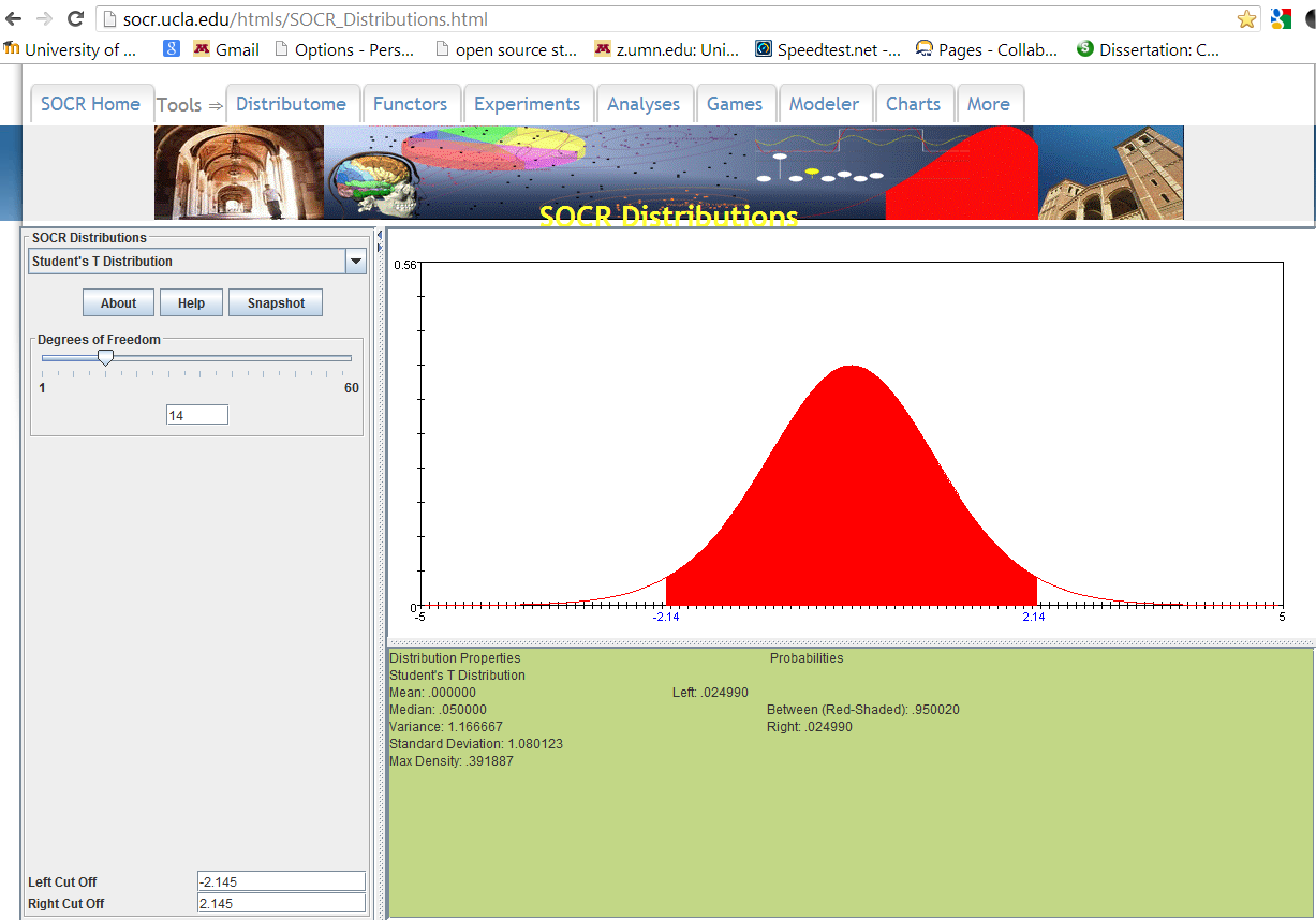
http://socr.ucla.edu/htmls/SOCR_Distributions.html has in the dropdown menu for SOCR distribution the normal distribution and for a Student’s t-distribution. For a normal distribution, you will need to have your mean and standard deviation and again your right and left cut off values (which in this case will be your critical values). For a Student’s t-distribution, you will need to have degrees of freedom and again your right and left cut off values (which in this case will be your critical values). Below is a graph of the Student’s t-distribution. We have used the example from 8.6 Two column Model step by step example for this demonstration. The degrees of freedom were 14 and a 95% confidence interval. We used the t-table to determine the left and right cut off values. In this instance two tailed confidence interval of 95% with 14 degrees for freedom is minus and plus 2.145.

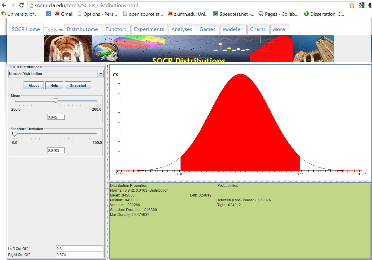
This next example is using the normal distribution for determining the confidence interval for a population proportion. The normal density curve here has the population proportion as the mean (p or p-hat) and the standard deviation (the square root of (p(1-p)/n). We have demonstrated the example 8.8 to show you how this looks in SOCR. For this problem the mean proportion was .842 and the critical z-value for a 95% confidence interval was ± 0.032 or (0.81, 0.874).

At your computer, try to use some of these tools to work out your homework problems or check homework that you have completed to see if the results are the same or similar.

Notification Switch
Would you like to follow the 'Collaborative statistics using spreadsheets' conversation and receive update notifications?