7.5 Labor-leisure choices  (Page 2/12)

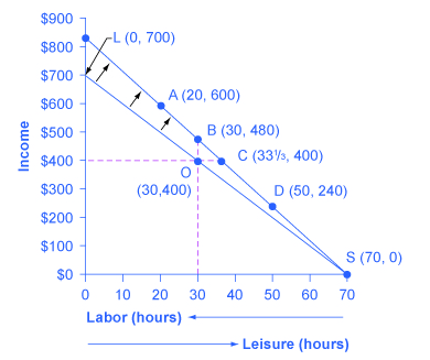
Vivian has 70 hours per week that she could devote either to work or to leisure, and her wage is $10/hour. The lower budget constraint in [link] shows Vivian’s possible choices. The horizontal axis of this diagram measures both leisure and labor, by showing how Vivian’s time is divided between leisure and labor. Hours of leisure are measured from left to right on the horizontal axis, while hours of labor are measured from right to left. Vivian will compare choices along this budget constraint, ranging from 70 hours of leisure and no income at point S to zero hours of leisure and $700 of income at point L. She will choose the point that provides her with the highest total utility. For this example, let’s assume that Vivian’s utility-maximizing choice occurs at O, with 30 hours of leisure, 40 hours of work, and $400 in weekly income.

How a rise in wages alters the utility-maximizing choice

For Vivian to discover the labor-leisure choice that will maximize her utility, she does not have to place numerical values on the total and marginal utility that she would receive from every level of income and leisure. All that really matters is that Vivian can compare, in her own mind, whether she would prefer more leisure or more income, given the tradeoffs she faces. If Vivian can say to herself: “I’d really rather work a little less and have more leisure, even if it means less income,” or “I’d be willing to work more hours to make some extra income,” then as she gradually moves in the direction of her preferences, she will seek out the utility-maximizing choice on her labor-leisure budget constraint.

Now imagine that Vivian’s wage level increases to $12/hour. A higher wage will mean a new budget constraint that tilts up more steeply; conversely, a lower wage would have led to a new budget constraint that was flatter. How will a change in the wage and the corresponding shift in the budget constraint affect Vivian’s decisions about how many hours to work?

Vivian’s choices of quantity of hours to work and income along her new budget constraint can be divided into several categories, using the dashed horizontal and vertical lines in [link] that go through her original choice (O). One set of choices in the upper-left portion of the new budget constraint involves more hours of work (that is, less leisure) and more income, at a point like A with 20 hours of leisure, 50 hours of work, and $600 of income (that is, 50 hours of work multiplied by the new wage of $12 per hour). A second choice would be to work exactly the same 40 hours, and to take the benefits of the higher wage in the form of income that would now be $480, at choice B. A third choice would involve more leisure and the same income at point C (that is, 33-1/3 hours of work multiplied by the new wage of $12 per hour equals $400 of total income). A fourth choice would involve less income and much more leisure at a point like D, with a choice like 50 hours of leisure, 20 hours of work, and $240 in income.