| << Chapter < Page | Chapter >> Page > |

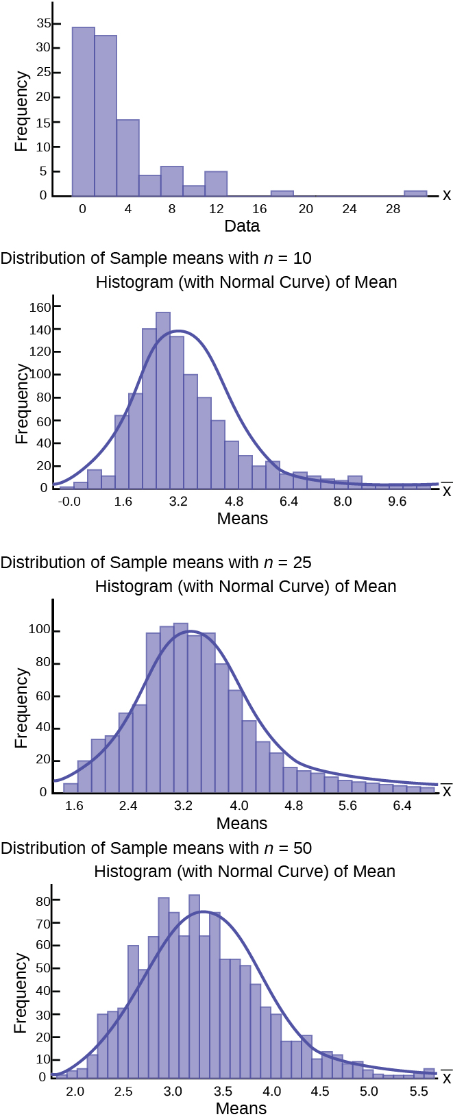
The Central Limit Theorem provides more than the proof that the sampling distribution of means is normally distributed. It also provides us with the mean and standard deviation of this distribution. Further, as discussed above, the expected value of the mean, , is equal to the mean of the population of the original data which is what we are interested in estimating from the sample we took. We have already inserted this conclusion of the Central Limit Theorem into the formula we use for standardizing from the sampling distribution to the standard normal distribution. And finally, the Central Limit Theorem has also provided the standard deviation of the sampling distribution, , and this is critical to have to calculate probabilities of values of the new random variable, .
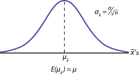
[link] shows a sampling distribution. The mean has been marked on the horizontal axis of the 's and the standard deviation has been written to the right above the distribution. Notice that the standard deviation of the sampling distribution is the original standard deviation of the population, divided by the sample size. We have already seen that as the sample size increases the sampling distribution becomes closer and closer to the normal distribution. As this happens, the standard deviation of the sampling distribution changes in another way; the standard deviation decreases as n increases. At very very large n, the standard deviation of the sampling distribution becomes very small and at infinity it collapses on top of the population mean. This is what it means that the expected value of is the population mean, µ.

At non-extreme values of n,this relationship between the standard deviation of the sampling distribution and the sample size plays a very important part in our ability to estimate the parameters we are interested in.
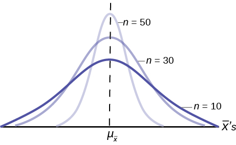
[link] shows three sampling distributions. The only change that was made is the sample size that was used to get the sample means for each distribution. As the sample size increases, n goes from 10 to 30 to 50, the standard deviations of the respective sampling distributions decrease because the sample size is in the denominator of the standard deviations of the sampling distributions.

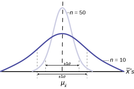
The implications for this are very important. [link] shows the effect of the sample size on the confidence we will have in our estimates. These are two sampling distributions from the same population. One sampling distribution was created with samples of size 10 and the other with samples of size 50. All other things constant, the sampling distribution with sample size 50 has a smaller standard deviation that causes the graph to be higher and narrower. The important effect of this is that for the same probability of one standard deviation from the mean, this distribution covers much less of a range of possible values than the other distribution. One standard deviation is marked on the axis for each distribution. This is shown by the two arrows that are plus or minus one standard deviation for each distribution. If the probability that the true mean is one standard deviation away from the mean, then for the sampling distribution with the smaller sample size, the possible range of values is much greater. A simple question is, would you rather have a sample mean from the narrow, tight distribution, or the flat, wide distribution as the estimate of the population mean? Your answer tells us why people intuitively will always choose data from a large sample rather than a small sample. The sampling mean they are getting is coming from a more compact distribution. This concept will be the foundation for what will be called level of confidence in the next unit.

The Central Limit Theorem can be used to illustrate the law of large numbers. The law of large numbers states that the larger the sample size you take from a population, the closer the sample mean gets to μ .
Use the following information to answer the next ten exercises: A manufacturer produces 25-pound lifting weights. The lowest actual weight is 24 pounds, and the highest is 26 pounds. Each weight is equally likely so the distribution of weights is uniform. A sample of 100 weights is taken.
Draw the graph from [link]
Find the probability that the mean actual weight for the 100 weights is greater than 25.2.
0.0003
Draw the graph from [link]
Find the 90 th percentile for the mean weight for the 100 weights.
25.07
Draw the graph from [link]
Draw the graph from [link]
Find the 90 th percentile for the total weight of the 100 weights.
2,507.40
Draw the graph from [link]
Use the following information to answer the next five exercises: The length of time a particular smartphone's battery lasts follows an exponential distribution with a mean of ten months. A sample of 64 of these smartphones is taken.
What is the distribution for the length of time one battery lasts?
What is the distribution for the mean length of time 64 batteries last?
N
What is the distribution for the total length of time 64 batteries last?
Find the probability that the sample mean is between seven and 11.
0.7799
Find the 80 th percentile for the total length of time 64 batteries last.
Find the IQR for the mean amount of time 64 batteries last.
1.69
Find the middle 80% for the total amount of time 64 batteries last.
Use the following information to answer the next eight exercises: A uniform distribution has a minimum of six and a maximum of ten. A sample of 50 is taken.
Find P ( Σx >420).
0.0072
Find the 90 th percentile for the sums.
Find the 15 th percentile for the sums.
391.54
Find the first quartile for the sums.
Find the third quartile for the sums.
405.51
Find the 80 th percentile for the sums.

Notification Switch
Would you like to follow the 'Introductory statistics' conversation and receive update notifications?