<< Chapter < Page Chapter >> Page >

Use of m-procedures to compare

We have two m-procedures to make the comparisons. First, we consider approximation of the
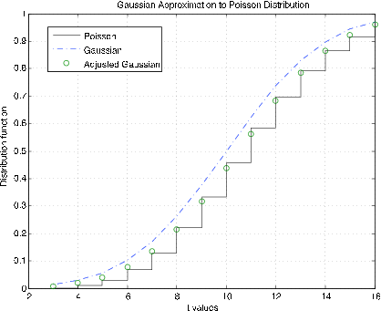
A graph of a Gaussian Approximation to Poisson Distribution.The x-axis displays the values for t ranging from 2-16 while the y-axis represents the values of distribution functions ranging from 0-1. There are two plotted distributions. The Poisson approximation is represented stepwise with green circles present near the external right angles indicating the position of the adjusted Gaussian approximation. The Gaussian approximation is represented with a dashed blue line and corresponds roughly to the green circles. A graph of a Gaussian Approximation to Poisson Distribution.The x-axis displays the values for t ranging from 2-16 while the y-axis represents the values of distribution functions ranging from 0-1. There are two plotted distributions. The Poisson approximation is represented stepwise with green circles present near the external right angles indicating the position of the adjusted Gaussian approximation. The Gaussian approximation is represented with a dashed blue line and corresponds roughly to the green circles.
Gaussian approximation to the Poisson distribution function μ = 10 .
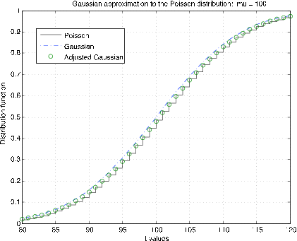
A graph of a Gaussian Approximation to Poisson distribution for  mu=100. The x-axis displays the values for t ranging from 80-120 while the y-axis represents the values of distribution functions ranging from 0-1. There are two plotted distributions. The Poisson approximation is represented stepwise with green circles present near the external right angles indicating the position of the adjusted Gaussian approximation. The Gaussian approximation is represented with a dashed blue line and corresponds roughly to the green circles. A graph of a Gaussian Approximation to Poisson distribution for  mu=100. The x-axis displays the values for t ranging from 80-120 while the y-axis represents the values of distribution functions ranging from 0-1. There are two plotted distributions. The Poisson approximation is represented stepwise with green circles present near the external right angles indicating the position of the adjusted Gaussian approximation. The Gaussian approximation is represented with a dashed blue line and corresponds roughly to the green circles.
Gaussian approximation to the Poisson distribution function μ = 100 .

Poisson ( μ ) distribution. The m-procedure poissapp calls for a value of μ , selects a suitable range about k = μ and plots the distribution function for the Poisson distribution (stairs) and the normal (gaussian) distribution (dash dot) for N ( μ , μ ) . In addition, the continuity correction is applied to the gaussian distribution at integer values (circles). [link] shows plots for μ = 10 . It is clear that the continuity correction provides a much better approximation. The plots in [link] are for μ = 100 . Here the continuity correction provides the better approximation, but not by as much as for the smaller μ .
A graph of a Gaussian Approximation to Poisson distribution for  mu=100. The x-axis displays the values for t ranging from 80-120 while the y-axis represents the values of distribution functions ranging from 0-1. There are two plotted distributions. The Poisson approximation is represented stepwise with green circles present near the external right angles indicating the position of the adjusted Gaussian approximation. The Gaussian approximation is represented with a dashed blue line and corresponds roughly to the green circles. A graph of a Gaussian Approximation to Poisson distribution for  mu=100. The x-axis displays the values for t ranging from 80-120 while the y-axis represents the values of distribution functions ranging from 0-1. There are two plotted distributions. The Poisson approximation is represented stepwise with green circles present near the external right angles indicating the position of the adjusted Gaussian approximation. The Gaussian approximation is represented with a dashed blue line and corresponds roughly to the green circles.
Poisson and Gaussian approximation to the binomial: n = 1000, p = 0.03.
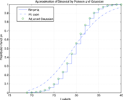
A graph of an Approximation of Binomial by Poisson and Gaussian. The x-axis displays the values for t ranging from 15-40 while the y-axis represents the values of distribution functions ranging from 0-1. There are two plotted distributions. The Binomial approximation is represented stepwise with green circles present near the external right angles indicating the position of the adjusted Gaussian approximation. The Poisson approximation is represented with a dashed blue line and corresponds roughly to the green circles, except at the top right of the graph where the Poisson distribution falls below the Binomial. A graph of an Approximation of Binomial by Poisson and Gaussian. The x-axis displays the values for t ranging from 15-40 while the y-axis represents the values of distribution functions ranging from 0-1. There are two plotted distributions. The Binomial approximation is represented stepwise with green circles present near the external right angles indicating the position of the adjusted Gaussian approximation. The Poisson approximation is represented with a dashed blue line and corresponds roughly to the green circles, except at the top right of the graph where the Poisson distribution falls below the Binomial.
Poisson and Gaussian approximation to the binomial: n = 50, p = 0.6.

The m-procedure bincomp compares the binomial, gaussian, and Poisson distributions. It calls for values of n and p , selects suitable k values, and plots the distribution function for the binomial, a continuous approximation to the distribution function for the Poisson,and continuity adjusted values of the gaussian distribution function at the integer values. [link] shows plots for n = 1000 , p = 0 . 03 . The good agreement of all three distribution functions is evident. [link] shows plots for n = 50 , p = 0 . 6 . There is still good agreement of the binomial and adjusted gaussian. However, the Poisson distribution does nottrack very well. The difficulty, as we see in the unit Variance , is the difference in variances— n p q for the binomial as compared with n p for the Poisson.

Approximation of a real random variable by simple random variables

Simple random variables play a significant role, both in theory and applications. In the unit Random Variables , we show how a simple random variable is determined by the set of points on the real line representingthe possible values and the corresponding set of probabilities that each of these values is taken on. This describes the distribution of the random variable and makes possible calculations of eventprobabilities and parameters for the distribution.

A continuous random variable is characterized by a set of possible values spread continuously over an interval or collection of intervals. In this case, the probability is also spread smoothly. The distributionis described by a probability density function, whose value at any point indicates "the probability per unit length" near the point. A simple approximation is obtained by subdividing an interval whichincludes the range (the set of possible values) into small enough subintervals that the density is approximately constant over each subinterval. A point in each subinterval is selected and is assigned the probabilitymass in its subinterval. The combination of the selected points and the corresponding probabilities describes the distribution of an approximating simple random variable. Calculations based on thisdistribution approximate corresponding calculations on the continuous distribution.

Get Jobilize Job Search Mobile App in your pocket Now!

Get it on Google Play Download on the App Store Now


Source:  OpenStax, Applied probability. OpenStax CNX. Aug 31, 2009 Download for free at http://cnx.org/content/col10708/1.6
Google Play and the Google Play logo are trademarks of Google Inc.

Notification Switch

Would you like to follow the 'Applied probability' conversation and receive update notifications?

Ask