| << Chapter < Page | Chapter >> Page > |
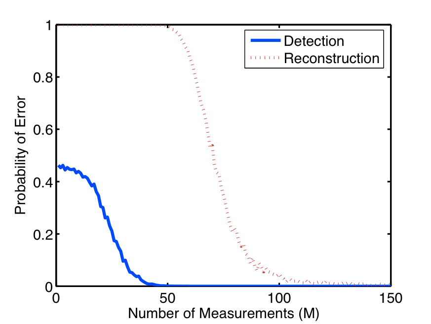
In the case where the class of signals of interest corresponds to a low dimensional subspace, a truncated, simplified sparse approximation can be applied as a detection algorithm; this has been dubbed as IDEA [link] . In simple terms, the algorithm will mark a detection when a large enough amount of energy from the measurements lies in the projected subspace. Since this problem does not require accurate estimation of the signal values, but rather whether it belongs in the subspace of interest or not, the number of measurements necessary is much smaller than that required for reconstruction, as shown in [link] .


Similarly, random projections have long been used for a variety of classification and clustering problems. The Johnson-Lindenstrauss Lemma is often exploited in this setting to compute approximate nearest neighbors, which is naturally related to classification. The key result that randomprojections result in an isometric embedding allows us to generalize this work to several new classification algorithms and settings [link] .
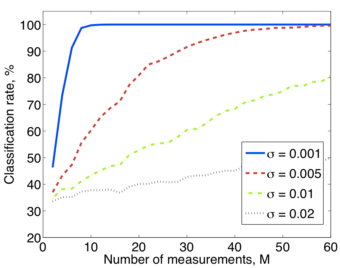
Classification can also be performed when more elaborate models are used for the different classes. Suppose the signal/image class of interest can be modeled as a low-dimensional manifold in the ambient space. In such case it can be shown that, even under random projections, certain geometric properties of the signal class are preserved up to a small distortion; for example, interpoint Euclidean ( ) distances are preserved [link] . This enables the design of classification algorithms in the projected domain. One such algorithm is known as the smashed filter [link] . As an example, under equal distribution among classes and a gaussian noise setting, the smashed filter is equivalent to building a nearest-neighbor (NN) classifier in the measurement domain. Further, it has been shown that for a dimensional manifold, measurements are sufficient to perform reliable compressive classification. Thus, the number of measurements scales as the dimension of the signal class, as opposed to the sparsity of the individual signal. Some example results are shown in [link] (a).


Consider a signal , and suppose that we wish to estimate some function but only observe the measurements , where is again an matrix. The data streaming community has previously analyzed this problem for many common functions, such as linear functions, norms, and histograms. These estimates are often based on so-called sketches , which can be thought of as random projections.
As an example, in the case where is a linear function, one can show that the estimation error (relative to the norms of and ) can be bounded by a constant determined by . This result holds for a wide class of random matrices, and can be viewed as a straightforward consequence of the same concentration of measure inequality that has proven useful for CS and in proving the JL Lemma [link] .
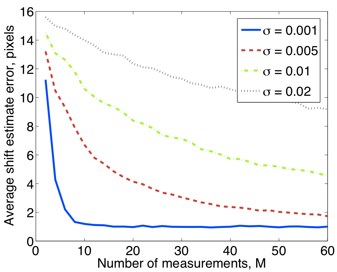
Parameter estimation can also be performed when the signal class is modeled as a low-dimensional manifold. Suppose an observed signal can be parameterized by a dimensional parameter vector , where . Then, it can be shown that with 0 measurements, the parameter vector can be obtained via multiscale manifold navigation in the compressed domain [link] . Some example results are shown in [link] (b).

Notification Switch
Would you like to follow the 'An introduction to compressive sensing' conversation and receive update notifications?