| << Chapter < Page | Chapter >> Page > |

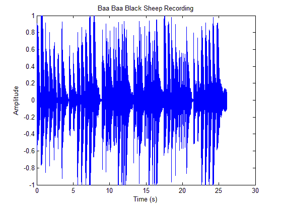
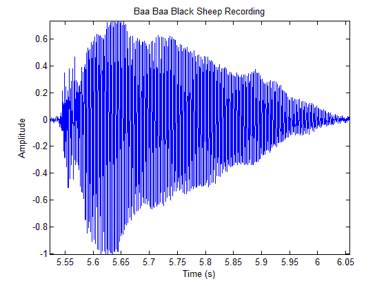
At first sight, we can see that note attacks are clearly defined by large spikes. Though these spikes are visually easy to identify, when we take a closer look at the signal, we see that it is fluctuating rapidly, meaning that there is a lot of high frequency content in each note. Thus, to identify the peaks of each note, we can’t simply look at all the high points or the points where the value of the data rises exponentially. We’ll have to do some pre-processing and filtering to identify the edges computationally.

We decided to try out a low-pass filter to smooth out the sharp changes in the song so all that’s left are smooth increases and decreases, where each rise and fall corresponds to a single note. First we decided that the length of the filter should be proportional to the sampling frequency, which fixes its length in time. Then we decided to try out a simple boxcar filter and convolve that with the square (i.e. the power) of our signal. It turned out that we decided to convolve it with a boxcar 3 times over, which is the same as convolve it once with 3 boxcars convolved together. Visually, this was our filter:

And here’s our smoothed signal superimposed on our original file:

We proceed to use MATLAB’s function “findpeaks.” We twiddled with parameters like the minimum height of the peaks listed and the minimum distance between peaks to ensure that small ripples in some attacks did not get counted twice. The algorithm then takes the distance between the peaks as the lengths of the notes.
There is a second part of the algorithm that calculates the beats per minute and attempts to characterize each note in terms of its beats, i.e. a half-note, quarter-note, eight-note, etc. This is done by finding the smallest interval, corresponding to the shortest note, and assumes all the note durations are multiples of this length. We assume the bpm of our song ranges from 100 bpm to 200 bpm – if we don’t, then we could say a quarter note at 80 bpm is the same as a half note at 160 bpm. There is a degree of tolerance (that can be varied) to determine whether two note durations correspond to the same note, as the lengths of each note we get are not perfect multiples of each other. This mapping works very well for synthesized music, but is not practical for live recordings of music or overtly rubato music, as the length of each beat is not fixed.
Below is a sample output of our note divider function where data1 is a synthesized audio file of Hot Cross Buns, fs is the sampling frequency of 44.1kHz, bpm is the beats per minute, notes is the estimated length of each note, and notetimes has is the length of each note in samples:
[bpm, notes, notetimes] = notedivider(data1, fs)
| bpm | notes | note times |
| 120.8288 | 1.000 | 22754 |
| 1.000 | 21846 | |
| 2.000 | 43401 | |
| 1.000 | 22925 | |
| 1.000 | 21847 | |
| 2.000 | 43819 | |
| 0.500 | 10987 | |
| 0.500 | 11054 | |
| 0.500 | 10563 | |
| 0.500 | 11136 | |
| 0.500 | 10793 | |
| 0.500 | 11321 | |
| 0.500 | 10803 | |
| 0.500 | 10938 | |
| 1.000 | 23082 | |
| 1.000 | 21847 | |
| 3.000 | 61401 |
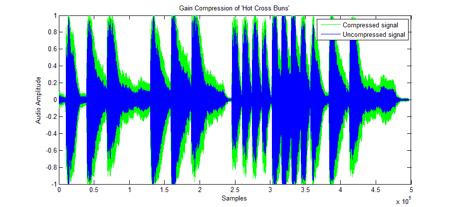
Below is our algorithm. x[n]is our input signal, y[n] is the compressed signal, lambda is a parameter greater than 1. Increasing it equalizes the note heights more and more. For our implementation we used a lambda value of 2.

After compression, we smooth the signal using a thrice convolved boxcar filter. This will produce a single continuous line that outlines the edge of the signal. This makes detecting the onset of a note easier by allowing us to locate the peak of a note with more ease.

Notification Switch
Would you like to follow the 'Elec 301 projects fall 2013' conversation and receive update notifications?