| << Chapter < Page | Chapter >> Page > |
By the end of this section, you will be able to:
Let’s begin this discussion with a single economic event. It might be an event that affects demand, like a change in income, population, tastes, prices of substitutes or complements, or expectations about future prices. It might be an event that affects supply, like a change in natural conditions, input prices, or technology, or government policies that affect production. How does this economic event affect equilibrium price and quantity? We will analyze this question using a four-step process.
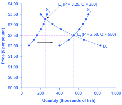
Step 1. Draw a demand and supply model before the economic change took place. To establish the model requires four standard pieces of information: The law of demand, which tells us the slope of the demand curve; the law of supply, which gives us the slope of the supply curve; the shift variables for demand; and the shift variables for supply. From this model, find the initial equilibrium values for price and quantity.
Step 2. Decide whether the economic change being analyzed affects demand or supply. In other words, does the event refer to something in the list of demand factors or supply factors?
Step 3. Decide whether the effect on demand or supply causes the curve to shift to the right or to the left, and sketch the new demand or supply curve on the diagram. In other words, does the event increase or decrease the amount consumers want to buy or producers want to sell?
Step 4. Identify the new equilibrium and then compare the original equilibrium price and quantity to the new equilibrium price and quantity.
Let’s consider one example that involves a shift in supply and one that involves a shift in demand. Then we will consider an example where both supply and demand shift.
In the summer of 2000, weather conditions were excellent for commercial salmon fishing off the California coast. Heavy rains meant higher than normal levels of water in the rivers, which helps the salmon to breed. Slightly cooler ocean temperatures stimulated the growth of plankton, the microscopic organisms at the bottom of the ocean food chain, providing everything in the ocean with a hearty food supply. The ocean stayed calm during fishing season, so commercial fishing operations did not lose many days to bad weather. How did these climate conditions affect the quantity and price of salmon? [link] illustrates the four-step approach, which is explained below, to work through this problem. [link] provides the information to work the problem as well.

| Price per Pound | Quantity Supplied in 1999 | Quantity Supplied in 2000 | Quantity Demanded |
|---|---|---|---|
| $2.00 | 80 | 400 | 840 |
| $2.25 | 120 | 480 | 680 |
| $2.50 | 160 | 550 | 550 |
| $2.75 | 200 | 600 | 450 |
| $3.00 | 230 | 640 | 350 |
| $3.25 | 250 | 670 | 250 |
| $3.50 | 270 | 700 | 200 |

Notification Switch
Would you like to follow the 'Principles of macroeconomics' conversation and receive update notifications?