| << Chapter < Page | Chapter >> Page > |

While population size and density describe a population at one particular point in time, scientists must use demography to study the dynamics of a population. Demography is the statistical study of population changes over time: birth rates, death rates, and life expectancies. These population characteristics are often displayed in a life table.
Life tables provide important information about the life history of an organism and the life expectancy of individuals at each age. They are modeled after actuarial tables used by the insurance industry for estimating human life expectancy. Life tables may include the probability of each age group dying before their next birthday, the percentage of surviving individuals dying at a particular age interval (their mortality rate , and their life expectancy at each interval. An example of a life table is shown in [link] from a study of Dall mountain sheep, a species native to northwestern North America. Notice that the population is divided into age intervals (column A). The mortality rate (per 1000) shown in column D is based on the number of individuals dying during the age interval (column B), divided by the number of individuals surviving at the beginning of the interval (Column C) multiplied by 1000.
For example, between ages three and four, 12 individuals die out of the 776 that were remaining from the original 1000 sheep. This number is then multiplied by 1000 to give the mortality rate per thousand.
As can be seen from the mortality rate data (column D), a high death rate occurred when the sheep were between six months and a year old, and then increased even more from 8 to 12 years old, after which there were few survivors. The data indicate that if a sheep in this population were to survive to age one, it could be expected to live another 7.7 years on average, as shown by the life-expectancy numbers in column E.
| Life Table of Dall Mountain Sheep Data Adapted from Edward S. Deevey, Jr., “Life Tables for Natural Populations of Animals,” The Quarterly Review of Biology 22, no. 4 (December 1947): 283-314. | ||||
|---|---|---|---|---|
| A | B | C | D | E |
| Age interval (years) | Number dying in age interval out of 1000 born | Number surviving at beginning of age interval out of 1000 born | Mortality rate per 1000 alive at beginning of age interval | Life expectancy or mean lifetime remaining to those attaining age interval |
| 0–0.5 | 54 | 1000 | 54.0 | 7.06 |
| 0.5–1 | 145 | 946 | 153.3 | — |
| 1–2 | 12 | 801 | 15.0 | 7.7 |
| 2–3 | 13 | 789 | 16.5 | 6.8 |
| 3–4 | 12 | 776 | 15.5 | 5.9 |
| 4–5 | 30 | 764 | 39.3 | 5.0 |
| 5–6 | 46 | 734 | 62.7 | 4.2 |
| 6–7 | 48 | 688 | 69.8 | 3.4 |
| 7–8 | 69 | 640 | 107.8 | 2.6 |
| 8–9 | 132 | 571 | 231.2 | 1.9 |
| 9–10 | 187 | 439 | 426.0 | 1.3 |
| 10–11 | 156 | 252 | 619.0 | 0.9 |
| 11–12 | 90 | 96 | 937.5 | 0.6 |
| 12–13 | 3 | 6 | 500.0 | 1.2 |
| 13–14 | 3 | 3 | 1000 | 0.7 |
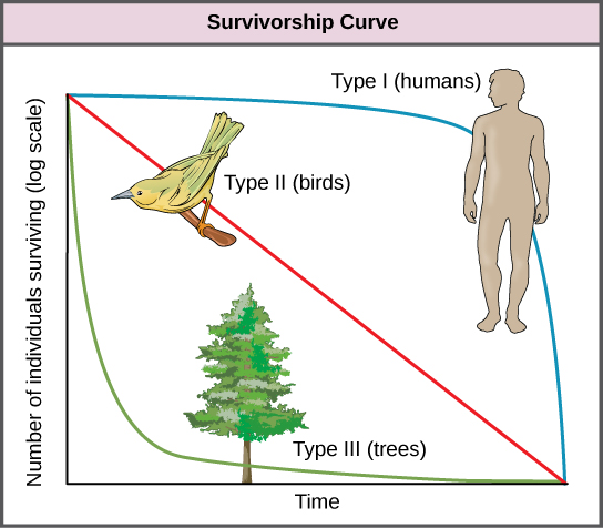
Another tool used by population ecologists is a survivorship curve , which is a graph of the number of individuals surviving at each age interval versus time. These curves allow us to compare the life histories of different populations ( [link] ). There are three types of survivorship curves. In a type I curve, mortality is low in the early and middle years and occurs mostly in older individuals. Organisms exhibiting a type I survivorship typically produce few offspring and provide good care to the offspring increasing the likelihood of their survival. Humans and most mammals exhibit a type I survivorship curve. In type II curves, mortality is relatively constant throughout the entire life span, and mortality is equally likely to occur at any point in the life span. Many bird populations provide examples of an intermediate or type II survivorship curve. In type III survivorship curves, early ages experience the highest mortality with much lower mortality rates for organisms that make it to advanced years. Type III organisms typically produce large numbers of offspring, but provide very little or no care for them. Trees and marine invertebrates exhibit a type III survivorship curve because very few of these organisms survive their younger years, but those that do make it to an old age are more likely to survive for a relatively long period of time.

Populations are individuals of a species that live in a particular habitat. Ecologists measure characteristics of populations: size, density, and distribution pattern. Life tables are useful to calculate life expectancies of individual population members. Survivorship curves show the number of individuals surviving at each age interval plotted versus time.

Notification Switch
Would you like to follow the 'Nsc 1406: contemporary biology' conversation and receive update notifications?