| << Chapter < Page | Chapter >> Page > |
Here is an example of using the Excel program to run a regression for a particular specific case: estimating the demand for bricks. These data can be found in the provided Excel file. Begin by downloading these data into an Excel spreadsheet. Because of the quirky way Excel allows the data to be entered into the regression package it is best to have the independent variables, price of bricks and income next to each other as it is here.
Once your data are entered into the spreadsheet it is always good to look at the data. Examine the range, the means and the standard deviations. Use your understanding of descriptive statistics from the very first part of this course. In large data sets you will not be able to “scan” the data. The Analysis ToolPac makes it easy to get the range, mean and standard deviations. You can also quickly get correlations among the variables. Examine for outliers. In this example if you had a year where the price of bricks was $9.00 or $2.00 we should be suspicious. These values are several standard deviations from the mean and thus have a very low probability of coming from this distribution. Review the history. Did something happen? Was here a labor strike, change in import fees, something that makes these unusual conditions? Do not take the data without question. There may have been a typo somewhere, who knows without review.
The data gathered was determined by the model that is being tested. This should always be the case. One is not doing inferential statistics by throwing a mountain of data into a computer and asking the machine for a theory. Theory first, tests follow. In this case the theory of consumer demand posits that the quantity of a good demanded is inversely related to its price and is positively related to income. These data are national average prices and income is the nation’s per capita income. Consumption is national demand for bricks. These are time series data; we are tracking the brick market for the United States from 1982-2010.
We are trying to create a demand curve, which we know from economic theory shows how variables effect how much of a good gets consumed. We expect to see a negative relationship between price and quantity, i.e. as price increases then quantity demanded decreases. Similarly, we expect to see a positive relationship between income and quantity demanded. We expect these results because that is what is predicted by a hundred years of economic theory and research. Essentially we are testing this century-old hypothesis. Quantity demanded will be our Y variable, and Income and Price will be our two X variables.
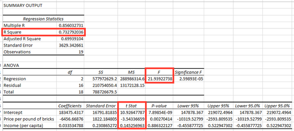
Go to the regression window, enter the data and select 95% confidence level and click “OK”. You can include the labels in the input range but be sure to click the “labels” box on the main regression page if you do.
The output should show up automatically on a new worksheet.

Titled as “Summary of Output”, the R-Square is the strength of the correlation between Y and X 1 and X 2 taken as a group. Our R-square, adjusted for degrees of freedom, of 0.699 means that 70% of the variation in Y, demand for bricks, can be explained by variations in X 1 and X 2 , Price and Income. Considering that bricks are an input in construction, omitted variables that are related to construction might explain the other 30% of the variation. This is a possible research topic.

Notification Switch
Would you like to follow the 'Introductory statistics' conversation and receive update notifications?