| << Chapter < Page | Chapter >> Page > |
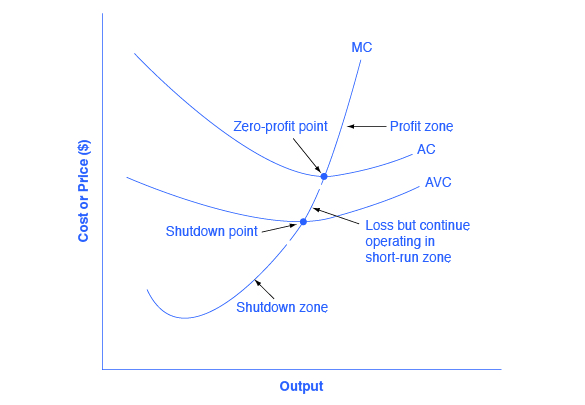
The average cost and average variable cost curves divide the marginal cost curve into three segments, as shown in [link] . At the market price, which the perfectly competitive firm accepts as given, the profit-maximizing firm chooses the output level where price or marginal revenue, which are the same thing for a perfectly competitive firm, is equal to marginal cost: P = MR = MC.

First consider the upper zone, where prices are above the level where marginal cost (MC) crosses average cost (AC) at the zero profit point. At any price above that level, the firm will earn profits in the short run. If the price falls exactly on the zero profit point where the MC and AC curves cross, then the firm earns zero profits. If a price falls into the zone between the zero profit point, where MC crosses AC, and the shutdown point, where MC crosses AVC, the firm will be making losses in the short run—but since the firm is more than covering its variable costs, the losses are smaller than if the firm shut down immediately. Finally, consider a price at or below the shutdown point where MC crosses AVC. At any price like this one, the firm will shut down immediately, because it cannot even cover its variable costs.
For a perfectly competitive firm, the marginal cost curve is identical to the firm’s supply curve starting from the minimum point on the average variable cost curve. To understand why this perhaps surprising insight holds true, first think about what the supply curve means. A firm checks the market price and then looks at its supply curve to decide what quantity to produce. Now, think about what it means to say that a firm will maximize its profits by producing at the quantity where P = MC. This rule means that the firm checks the market price, and then looks at its marginal cost to determine the quantity to produce—and makes sure that the price is greater than the minimum average variable cost. In other words, the marginal cost curve above the minimum point on the average variable cost curve becomes the firm’s supply curve.
Watch this video that addresses how drought in the United States can impact food prices across the world. (Note that the story on the drought is the second one in the news report; you need to let the video play through the first story in order to watch the story on the drought.)

Notification Switch
Would you like to follow the 'Openstax microeconomics in ten weeks' conversation and receive update notifications?