| << Chapter < Page | Chapter >> Page > |
A classic problem that explores scalable parallel processing is the heat flow problem. The physics behind this problem lie in partial differential equations.
We will start with a one-dimensional metal plate (also known as a rod), and move to a two-dimensional plate in later examples. We start with a rod that is at zero degrees celsius. Then we place one end in 100 degree steam and the other end in zero degree ice. We want to simulate how the heat flows from one end to another. And the resulting temperatures along points on the metal rod after the temperature has stabilized.
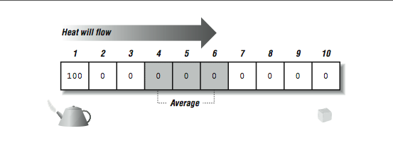
To do this we break the rod into 10 segments and track the temperature over time for each segment. Intuitively, within a time step, the next temperature of a portion of the plate is an average of the surrounding temperatures. Given fixed temperatures at some points in the rod, the temperatures eventually converge to a steady state after sufficient time steps. [link] shows the setup at the beginning of the simulation.

A simplistic implementation of this is as follows:
PROGRAM HEATROD
      PARAMETER(MAXTIME=200)INTEGER TICKS,I,MAXTIME
      REAL*4 ROD(10)ROD(1) = 100.0
      DO I=2,9ROD(I) = 0.0
      ENDDOROD(10) = 0.0
      DO TICKS=1,MAXTIMEIF ( MOD(TICKS,20) .EQ. 1 ) PRINT 100,TICKS,(ROD(I),I=1,10)
        DO I=2,9ROD(I) = (ROD(I-1) + ROD(I+1) ) / 2
        ENDDOENDDO
100   FORMAT(I4,10F7.2)END
The output of this program is as follows:
% f77 heatrod.f
heatrod.f:MAIN heatrod:
% a.out1 100.00   0.00   0.00   0.00   0.00   0.00   0.00   0.00   0.00  0.00
  21 100.00  87.04  74.52  62.54  51.15  40.30  29.91  19.83   9.92  0.0041 100.00  88.74  77.51  66.32  55.19  44.10  33.05  22.02  11.01  0.00
  61 100.00  88.88  77.76  66.64  55.53  44.42  33.31  22.21  11.10  0.0081 100.00  88.89  77.78  66.66  55.55  44.44  33.33  22.22  11.11  0.00
 101 100.00  88.89  77.78  66.67  55.56  44.44  33.33  22.22  11.11  0.00121 100.00  88.89  77.78  66.67  55.56  44.44  33.33  22.22  11.11  0.00
 141 100.00  88.89  77.78  66.67  55.56  44.44  33.33  22.22  11.11  0.00161 100.00  88.89  77.78  66.67  55.56  44.44  33.33  22.22  11.11  0.00
 181 100.00  88.89  77.78  66.67  55.56  44.44  33.33  22.22  11.11  0.00%
Clearly, by Time step 101, the simulation has converged to two decimal places of accuracy as the numbers have stopped changing. This should be the steady-state approximation of the temperature at the center of each segment of the bar.
Now, at this point, astute readers are saying to themselves, "Um, don't look now, but that loop has a flow dependency." You would also claim that this won't even parallelize a little bit. It is so bad you can't even unroll the loop for a little instruction-level parallelism!
A person familiar with the theory of heat flow will also point out that the above loop doesn't exactly implement the heat flow model. The problem is that the values on the right side of the assignment in the ROD loop are supposed to be from the previous time step, and that the value on the left side is the next time step. Because of the way the loop is written, the ROD(I-1) value is from the next time step, as shown in [link] .

Notification Switch
Would you like to follow the 'High performance computing' conversation and receive update notifications?