| << Chapter < Page | Chapter >> Page > |
A common way to determine similarity is to compute the normalized correlation between two signals (as shown in (7.1)); here, d represents the data segment, σ 2 represents the variance of the signal, and γ is the normalized correlation value Lewis, J.P., Fast Normalized Cross Correlation, Vision Interface , 1995, pp. 120-123 . The multiplication of the demeaned data segments is an element by element multiplication. A common correlation threshold used for similarity in signal processing applications is 95%. It is interesting to note that the normalized correlation value for two1 and two2 is approximately 32%; this value is remarkably low.
| (7.1) |
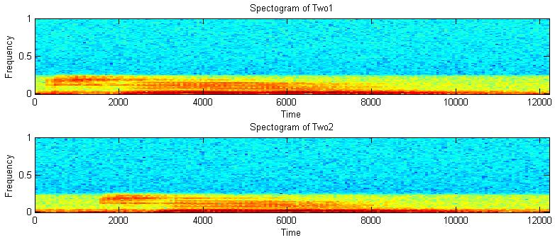
We get of hint of the similarities by observing a spectrogram of the two signals, shown in figure 7.1. By eye, we see that the two signals show similar spectral content through the phrase. The “trick” will be getting the computer to recognize that these two sequences are the same, as our eye does.

Figure 7.1: Spectograms of Two1 and Two2.
We begin by computing the norm of the difference of the spectrums. The procedure for doing so is shown in figure 7.2. We analyze this procedure step by step below.
Figure 7.2: Procedure for computing the norm of the difference of the two signal spectrums.
N max is the maximum of the number of samples in the two data segments; i.e. . We zero pad the shorter signal such that it is the same length as the longer segment. We then calculate the FFT of the two zero-padded signals. Note that by computing the FFT of a zero-padded signal, we are effectively performing sinc interpolation in the frequency domain for the shorter sequence. The magnitudes of the spectrums for two1 and two2 are shown in figure 7.3.

Figure 7.3: Magnitude of the spectrums of two1 and two2 signals.
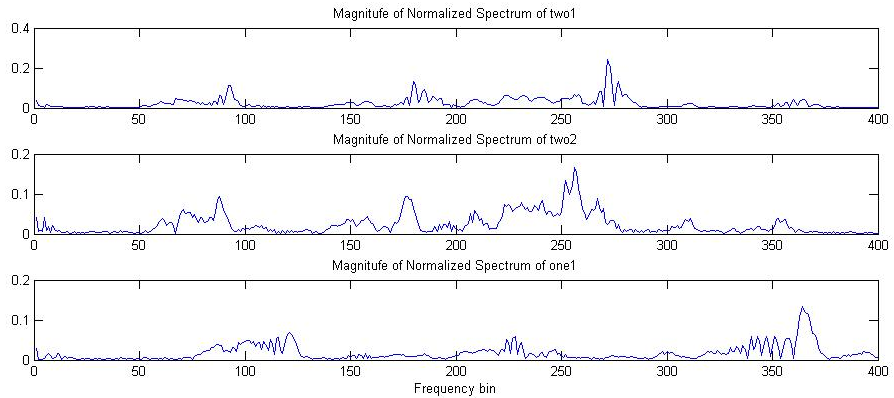
In figure 7.4, we zoom into the chart for improved resolution. We also show the spectrum of Nicholas saying the word “one” for comparison (this signal will be called one1 in this document). By eye, we are able to see that the spectrums of two1 and two2 are more similar to each other than the spectrum of one1 is.

Figure 7.4: Magnitude of the low frequency portion of spectrums of signals.
After identifying the relevant spectrums, we normalize them by the amount of energy in the spectrum. That is, we convert them according to the formula shown in (6.3), this time the data in question is the signal’s spectrum. According to Parseval’s theorem, this is equivalent to performing normalization in the time domain (of the zero padded signals). Figure 7.5 shows the normalized spectrums.

Figure 7.5: Magnitude of normalized spectrums for two1 and two2 signals.
Finally, we compute the element by element difference of the two spectrums and calculate the norm of this difference. For the “two” normalized spectrums used in this example, the norm of the difference was approximately 143%. After normalization, the energy in each individual spectrum is 1. Again, the energy in the difference signal is very high for two signals that are the “same”.
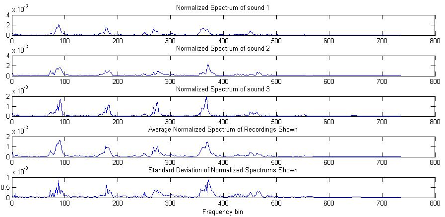
We begin to understand why when we statistically analyze a set of recordings of the same phrase. Shown in figure 7.6 is a set of spectrums for recordings made by Nicholas stating the word “one”. By observing these plots, we gain some intuition into what a word is. Let us call each bump in the spectrum a “pocket” of energy. We see that the word “one” has five pockets of energy. We see that different recordings have pockets located at approximately the same frequency bins, but that the shape of each pocket is different. Because of this difference, there is variability in the average of frequency bins with high average energy values. This variability is quantified through the standard deviation, shown in the last row of plot 7.6.

Figure 7.6: A depiction of spectrum magnitudes of several recordings of Nicholas saying the word “one”, the average and standard deviation of those spectrums.
We can use the L2 norm as a measure of the difference between the spectrum of two signals. We compute the L2 norm of Nicholas stating the word one (spectrum not shown) and the average “one” spectrum – the value is approximately 54%. When making the same comparison between the average spectrum and Nicholas stating the word “two”, the value becomes 75% - a percentage difference of approximately 36%. The deviation between the average “one” spectrum and Matt stating the word “one” is 62%.
We can take advantage of the knowledge of the variability of the signal in our comparison metric. To account for this variability, we can use a weighted L2 norm as our comparison metric. We define our weighted norm in (7.2).
| (7.2) |
This metric reduces the importance of mean data values with high variance, and increases the penalty for data values with low variance. We include an addition to a constant in the denominator to prevent division by 0, and we set this constant equal to since we notice that the noise in the normalized spectrum is around this level.
Using the weighted norm, we calculate a comparison metric between the average spectrum shown in figure 7.6, and a separate recording of Nicholas saying the word “one” to be 452. This seems like a high number, but it is no longer a physical quantity. We compare this value to the metric determined between the average spectrum shown in figure 7.6 and Nicholas saying the word “two”: 656. Notice that the difference in metric values is approximately 45%. The weighted norm value between the average spectrum shown in figure 7.6 and Matthew stating the word “one” is 691; a difference of approximately 53%.
Unfortunately, since the weighted norm value is not a physical quantity, we would require a large database of signals to determine the appropriate value for our threshold. In lieu of this, we will continue to use the L2 norm as our comparison metric.

Notification Switch
Would you like to follow the 'Analysis of speech signal spectrums using the l2 norm' conversation and receive update notifications?