| << Chapter < Page | Chapter >> Page > |
Thanks to the many resources available on the Internet, we were able to utilize Dirk-Jan Kroon’s Matlab adaptation of OpenSURF as the core function of the image processing part of our project.
OpenSurf returns a set of parameters for all the features above the set threshold. These parameters include x-position (scalar), y-position (scalar), scale (scalar), orientation (scalar), Laplacian (binary), and descriptor (vector). These parameters are put into a structure that is associated with each feature. Hence, if two hundred features are found to be above the threshold restriction, there will be two hundred structures in the output, each with cells such as x, y, and etc. The descriptors, however, are essential to feature matching between two images.
With the help of the example code also written by Kroon, we understood how to find matches between all of the features found and returned by the function OpenSurf.
If two images, I1 and I2, are processed by OpenSurf (I1 is the test image, while I2 is the template), two structures, T1 and T2, are returned. In order to match the features, the descriptor for each feature in the template needs to be compared to the descriptor for each feature in the test image (or the other way around). To do so, descriptors need to be extracted and put into a matrix for convenient usage. Kroon’s way of doing this is by making each descriptor a column vector and augmenting all such vectors into a matrix with dimensions “length of descriptor × number of features”. After doing this we will have two matrices, D1 and D2. To compare two vectors in multidimensional space, one would naturally think about least-squares-error, and this is indeed how the matching is done.
To avoid a nested for loop and increase computational speed, one column vector from D1 is taken at a time and is replicated (by tiling) into a matrix of the size of D2; then the least squares can be done in a matrix. Entry-wise differences are calculated between the newly constructed matrix and D2, and then the entry-wise square is taken. Each column is then summed and a distance error vector is generated. Next, we take the minimum distance and record the feature number from both I1 and I2 of the associated distance. After all the found features for D1 are compared with those of D2, a nice minimum distance vector is generated. From here it is quite easy to rank the similarity of the matches based on the minimum distance.
Of course not all matched features will be used. On one hand it is sufficient to have just a couple of matched points to find the same object. On the other hand, not all found features above the threshold are good matches. They might just be distinct features generated by OpenSurf, but might end up not matching anything on our target at all; in fact, they might just be a similar contour in a complex background. We call these features “astray points” because later when we try to pin down the center of the object, they introduce lots of error. The number of points that are used is set to be a variable so as to introduce some flexibility.
After selecting the eight best matches (the number we chose), we can use their feature number to access their individual information, such as position, in each picture.
Once we figure out how to find the matches and extract their relevant information, we need to calculate the data for our sound generation module. In a dance, it is the relative position of the body parts, their moving speed, and orientation that convey the most information; as a result, our first goal is to find out the position of the object’s center, how fast the center of the object is moving, if it is skewed, and how fast it is rotating.
We took an easy approach to calculate the center of the tracked object. The center is calculated by averaging the x and y indices with all the selected feature points. One might argue that this method is not robust against error. However, because of the special properties of the images we used (video, which means frames are blurry; distant objects, which lower the resolution even more), we can hardly tell if a point is an “astray point” or if the object is very close to the camera.


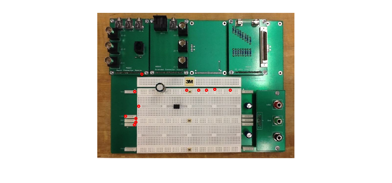
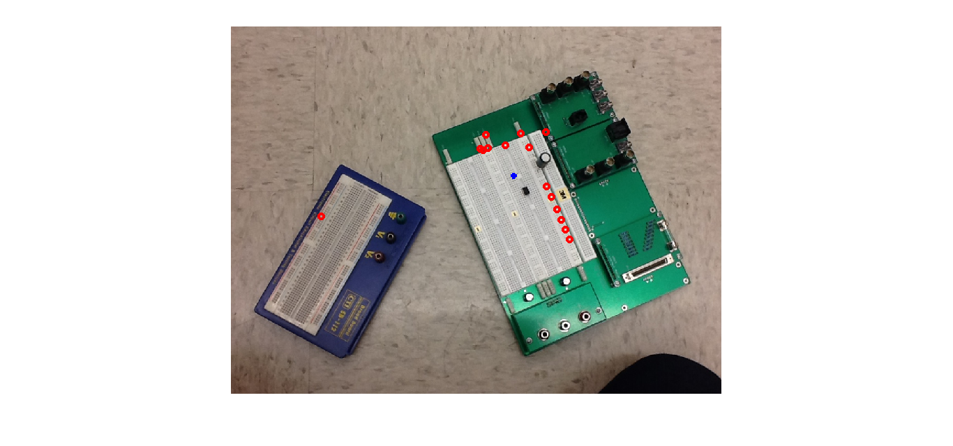
Figure (1) is the template, Figure (2) is the test image. The blue star is the calculated position of the target object. Notice that if the number of selected points is large enough, one astray point would not affect the result that much.

Orientation is not extracted from the feature descriptors; rather, it is calculated using matrix transformation (affine matrix).
Put the x and y positions from I1 into a column vector and augment all of these column vectors from different features into a matrix and call it X1. We can do the same thing for I2 and call it X2. Then we have
where A is the transformation matrix that contains information such as x and y scale and rotation angle. Thus,

where the S’s are scaling factors. To find out the angle, we can simply do X1/X2 and then divide the entry (1,2) by (2,2) of the resulting matrix, and it gives tan(a). We can then take the inverse tangent to find out the angle.
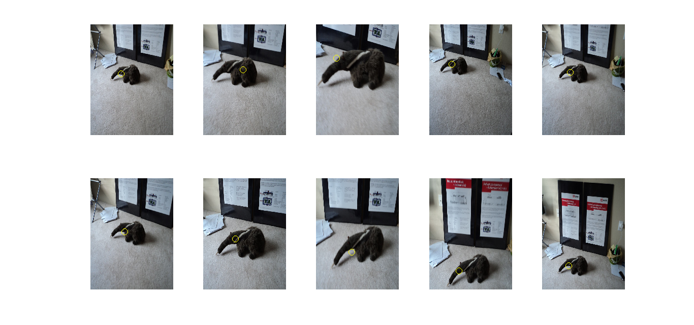
First, the video is recorded and completely loaded into MATLAB. We use one picture for the template; then we compare the template against each single frame using OpenSurf, and the position and orientation for the target object in that frame is calculated in the main for loop; this takes a while to run. Once the process is done, speed can be calculated. To ensure the same length of all output vectors, the first entries for translational velocity and rotational velocity are both set to 0. Later entries are calculated by the difference of position or angle (then divided by 30 because there are 30 frames per second) between two frames. The units for translational velocity are somewhat arbitrary because in this project we are not tracking the radial distance, and hence absolute speed cannot be calculated in a metric unit. The units for translational velocity are pixels per second; angular velocity is in radians per second.

Notification Switch
Would you like to follow the 'Dwts - dancing with three-dimensional sound' conversation and receive update notifications?