<< Chapter < Page Chapter >> Page >
The creation of this content was supported in some part by NSF grant 0538934.

If you have written parallel programs in G and have a multicore computer, CONGRATULATIONS!!! You have been successfully developing interactive parallel programs that execute in multicore PC processors.
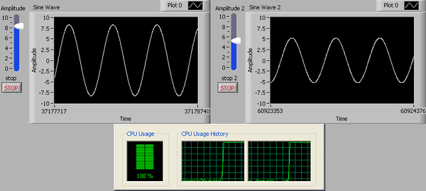
This screencap contain a diagram with two parallel graphs of sin waves and below these two graph is a CPU usage and CPU Usage History.
Interactive Multicore G Program

The following sections discuss some multicore programming techniques to improve the performance of G programs.

Data parallelism

Matrix multiplication is a compute intensive operation that can leverage data parallelism. [link] shows a G program with 8 sequential frames to demonstrate the performance improvement via data parallelism.
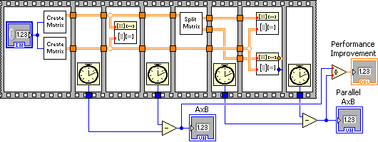
A complex diagram of a data parallelism.
Data Parallelism

The Create Matrix function generates a square matrix based of size indicated by Size containing random numbers between 0 and 1. The Create Matrix function is shown in [link] .

A diagram consisting of three box icons. From left to right you have a blue box labeled 'size'. The next element is two rectangles one large one underneath a smaller one. In the rectangles on the left of both are blue squares containing a 'N'and an 'i'. Blue lines point from the first icon to these blue squares. An orange line points from these rectangles to the third icon labeled 'matrix'.
Creating a Square Matrix

The Split Matrix function determines the number of rows in the matrix and shifts right the resulting number of rows by one (integer divide by 2). This value is used to split the input matrix into the top half and bottom half matrices. The Split Matrix function is shown in [link] .
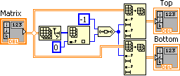
A diagram of a split matrix into top and bottom. The diagram consist of an icon labeled matrix. Two orange lines split off from the icon and go around a center icon to connect to two rectangles which then leads to two parallel icons labeled top and bottom.
Split Matrix into Top&Bottom
Sequence Frame Operation Description
First Frame Generates two square matrices initialized with random numbers
Second Frame Records start time for single core matrix multiply
Third Frame Performs single core matrix multiply
Fourth Frame Records stop time of single core matrix multiply
Fifth Frame Splits the matrix into top and bottom matrices
Sixth Frame Records start time for multicore matrix multiply
Seventh Frame Performs multicore matrix multiply
Eighth Frame Records stop time of multicore matrix multiply

The rest of the calculations determine the execution time in milliseconds of the single core and multicore matrix multiply operations and the performance improvement of using data parallelism in a multicore computer.

The program was executed in a dual core 1.83 GHz laptop. The results are shown in [link] . By leveraging data parallelism, the same operation has nearly a 2x performance improvement. Similar performance benefits can be obtained with higher multicore processors
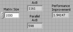
A diagram of Data Parallelism Performance Improvement. The diagram consists of four fields from left to right they are labeled: Matrix size with a value of 1000. Next a field 'AxB' with a value of 1161. Below this field is another field called 'parallel AxB' with a value of 598. The final field is labeled 'Performance Improvement' with a value of 1.94147.
Data Parallelism Performance Improvement

Task pipelining

A variety of applications require tasks to be programmed sequentially and continually iterate on these tasks. Most notably are telecommunications applications require simultaneous transmit and receive. In the following example, a simple telecommunications example illustrates how these sequential tasks can be pipelined to leverage multicore environments.

Consider the following simple modulation - demodulation example where a noisy signal is modulated transmitted and demodulated. A typical diagram is shown in [link] .

A diagram of sequential tasks. It consists of four icons in a row. The last icon is is surrounded in a orange box. Underneath this row is a stop button surrounded in great with a red button next to it. On the left corner there is an blue square containing an 'i'.
Sequential Tasks

Adding a shift register to the loop allows tasks to be pipelined and be executed in parallel in separate cores should they be available. Task pipelining is shown in [link] .
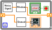
A diagram of 'Pipelined Task'. There are two paths of icons. The upper row of icons has two squares with a orange line connected them and then another orange line connects to the right side of the box. The bottom row begins with a orange line connected to the left side of the box and then extends to a gray box icon which is then connected via another orange line to graph icon that is in an orange box.
Pipelined Tasks

The program below times the sequential task and the pipelined tasks to establish its performance improvement when executed in multicore computers.

A diagram of a 'Task Pipelining Program Example'. The diagram is formed on a sort of film frame. There are also two rows. The upper from left to right is a box icon connected via an orange line to a box  with an 'N' with a '1000'in the upper left corner and an 'i' in the lower left. In the middle of this box are two horizontally oriented box icons. An orange line continues to the right to another box with the same setup as the previous, except the box icons are oriented vertically. The orange line continues through the upper box and ends to the right. The second row is below the other and consists of three clock icons linked by blue lines and then on the far right side there are arrows all pointing to three icons labeled from top to bottom 'pipelined', 'improvement', and 'sequential'.
Task Pipelining Program Example

[link] shows the results of running the above G program in a dual core 1.8 GHz laptop. Pipelining shows nearly 2x performance improvement.

A diagram of Performance Improvement due to Pipelining. There are three fields in this diagram. From left to right the fields are 'Sequential' with a value of 5953. Under that field is the another field labeled 'Pipelined' with a value of 3156. To the right of these two fields is the third and final field labeled 'improvement'with a value of 1.88625.
Pipelining Performance Improvement

Pipelining using feedback nodes

Feedback Nodes provide a storage mechanism between loop iterations. They are programmatically identical to the Shift Registers . Feedback Nodes consist of an Initializer Terminal and the Feedback Node itself (see [link] ).

A diagram of a feedback node. The diagram is arranged vertical with items top to bottom the phrase 'Feedback Node' with a orange line connecting it to an icon of an arrow above and icon of a black dot. An orange line connects that to the phrase 'Initializer Terminal'.
Feedback Node

To add a Feedback Node , right click on the Block Diagram window and select Feedback Node from the Functions>>Programming>>Structures pop-up menu. The direction of the Feedback Node can be changed by right clicking on the node and selecting Change Direction .
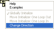
A diagram of menu listing over an arrow icon.
Feedback Node Direction

The diagram shown in [link] is programmatically identical to the diagram in [link] .

A diagram of 'Pipelining with Feedback Node'. The diagram is oriented horizontally, and from left to right the diagram consist of a box icon connected via an orange line to another box icon connected via a orange arrow to an arrow above a dot icon. The icon is also connected to the right via an orange line to a box icon which is connected to a graph icon. In the bottom left of the diagram is a blue square with an 'i' in is and on the bottom right is a 'stop' button icon.
Pipelining with Feedback Node

Similarly, the diagram in [link] is programmatically identical to that in [link] .

A diagram of a 'Task Pipelining Program Example'. The diagram is formed on a sort of film frame. There are also two rows. The upper from left to right is a box icon connected via an orange line to a box  with an 'N' with a '1000'in the upper left corner and an 'i' in the lower left. In the middle of this box are two horizontally oriented box icons. An orange line continues to the right to another box with the same setup as the previous, except between the two icons there is an orange arrow over a dot icon. The orange line continues through the boxes and icon and ends to the right. The second row is below the other and consists of three clock icons linked by blue lines and then on the far right side there are arrows all pointing to three icons labeled from top to bottom 'pipelined', 'improvement', and 'sequential'.
Pipelining Tasks with Feedback Nodes

Get Jobilize Job Search Mobile App in your pocket Now!

Get it on Google Play Download on the App Store Now


Source:  OpenStax, Introduction to g programming. OpenStax CNX. Mar 15, 2010 Download for free at http://cnx.org/content/col11192/1.1
Google Play and the Google Play logo are trademarks of Google Inc.

Notification Switch

Would you like to follow the 'Introduction to g programming' conversation and receive update notifications?

Ask