| << Chapter < Page | Chapter >> Page > |
where Qs is the amount of pizza producers will supply (i.e., quantity supplied).
Finally, suppose that the personal pizza market operates where supply equals demand, or
We now have a system of three equations and three unknowns (Qd, Qs, and P), which we can solve with algebra:
Since Qd = Qs, we can set the demand and supply equation equal to each other:
Subtracting 2 from both sides and adding 2P to both sides yields:
In other words, the price of each personal pizza will be $2. How much will consumers buy?
Taking the price of $2, and plugging it into the demand equation, we get:
So if the price is $2 each, consumers will purchase 12. How much will producers supply? Taking the price of $2, and plugging it into the supply equation, we get:
So if the price is $2 each, producers will supply 12 personal pizzas. This means we did our math correctly, since Qd = Qs.
Solving Models with Graphs
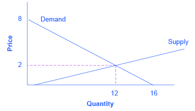
If algebra is not your forte, you can get the same answer by using graphs. Take the equations for Qd and Qs and graph them on the same set of axes as shown in [link] . Since P is on the vertical axis, it is easiest if you solve each equation for P. The demand curve is then P = 8 – 0.5Qd and the demand curve is P = –0.4 + 0.2Qs. Note that the vertical intercepts are 8 and –0.4, and the slopes are –0.5 for demand and 0.2 for supply. If you draw the graphs carefully, you will see that where they cross (Qs = Qd), the price is $2 and the quantity is 12, just like the algebra predicted.

We will use graphs more frequently in this book than algebra, but now you know the math behind the graphs.
Growth rates are frequently encountered in real world economics. A growth rate is simply the percentage change in some quantity. It could be your income. It could be a business’s sales. It could be a nation’s GDP. The formula for computing a growth rate is straightforward:
Suppose your job pays $10 per hour. Your boss, however, is so impressed with your work that he gives you a $2 per hour raise. The percentage change (or growth rate) in your pay is $2/$10 = 0.20 or 20%.
To compute the growth rate for data over an extended period of time, for example, the average annual growth in GDP over a decade or more, the denominator is commonly defined a little differently. In the previous example, we defined the quantity as the initial quantity—or the quantity when we started. This is fine for a one-time calculation, but when we compute the growth over and over, it makes more sense to define the quantity as the average quantity over the period in question, which is defined as the quantity halfway between the initial quantity and the next quantity. This is harder to explain in words than to show with an example. Suppose a nation’s GDP was $1 trillion in 2005 and $1.03 trillion in 2006. The growth rate between 2005 and 2006 would be the change in GDP ($1.03 trillion – $1.00 trillion) divided by the average GDP between 2005 and 2006 ($1.03 trillion + $1.00 trillion)/2. In other words:

Notification Switch
Would you like to follow the 'Principles of economics' conversation and receive update notifications?