30.4 Using fiscal policy to fight recession, unemployment, and  (Page 2/11)

Expansionary fiscal policy

Expansionary fiscal policy increases the level of aggregate demand, through either increases in government spending or reductions in taxes. Expansionary policy can do this by (1) increasing consumption by raising disposable income through cuts in personal income taxes or payroll taxes; (2) increasing investments by raising after-tax profits through cuts in business taxes; and (3) increasing government purchases through increased spending by the federal government on final goods and services and raising federal grants to state and local governments to increase their expenditures on final goods and services. Contractionary fiscal policy does the reverse: it decreases the level of aggregate demand by decreasing consumption, decreasing investments, and decreasing government spending, either through cuts in government spending or increases in taxes. The aggregate demand/aggregate supply model is useful in judging whether expansionary or contractionary fiscal policy is appropriate.

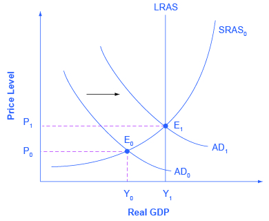
Consider first the situation in [link] , which is similar to the U.S. economy during the recession in 2008–2009. The intersection of aggregate demand (AD ₀ ) and aggregate supply (SRAS ₀ ) is occurring below the level of potential GDP as indicated by the LRAS curve. At the equilibrium (E ₀ ), a recession occurs and unemployment rises. In this case, expansionary fiscal policy using tax cuts or increases in government spending can shift aggregate demand to AD ₁ , closer to the full-employment level of output. In addition, the price level would rise back to the level P ₁ associated with potential GDP.

Expansionary fiscal policy

Should the government use tax cuts or spending increases, or a mix of the two, to carry out expansionary fiscal policy? After the Great Recession of 2008–2009 (which started, actually, in very late 2007), U.S. government spending rose from 19.6% of GDP in 2007 to 24.6% in 2009, while tax revenues declined from 18.5% of GDP in 2007 to 14.8% in 2009. The choice between whether to use tax or spending tools often has a political tinge. As a general statement, conservatives and Republicans prefer to see expansionary fiscal policy carried out by tax cuts, while liberals and Democrats prefer that expansionary fiscal policy be implemented through spending increases. The Obama administration and Congress passed an $830 billion expansionary policy in early 2009 involving both tax cuts and increases in government spending, according to the Congressional Budget Office. However, state and local governments, whose budgets were also hard hit by the recession, began cutting their spending—a policy that offset federal expansionary policy.