0.4 The expenditure-output model  (Page 12/16)

The size of the multiplier is determined by what proportion of the marginal dollar of income goes into taxes, saving, and imports. These three factors are known as “leakages,” because they determine how much demand “leaks out” in each round of the multiplier effect. If the leakages are relatively small, then each successive round of the multiplier effect will have larger amounts of demand, and the multiplier will be high. Conversely, if the leakages are relatively large, then any initial change in demand will diminish more quickly in the second, third, and later rounds, and the multiplier will be small. Changes in the size of the leakages—a change in the marginal propensity to save, the tax rate, or the marginal propensity to import—will change the size of the multiplier.

Calculating Keynesian Policy Interventions

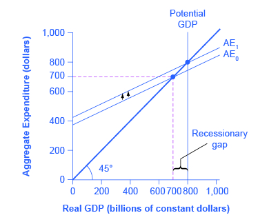
Returning to the original question: How much should government spending be increased to produce a total increase in real GDP of $100? If the goal is to increase aggregate demand by $100, and the multiplier is 2.13, then the increase in government spending to achieve that goal would be $100/2.13 = $47. Government spending of approximately $47, when combined with a multiplier of 2.13 (which is, remember, based on the specific assumptions about tax, saving, and import rates), produces an overall increase in real GDP of $100, restoring the economy to potential GDP of $800, as [link] shows.

The multiplier effect in an expenditure-output model

The multiplier effect is also visible on the Keynesian cross diagram. [link] shows the example we have been discussing: a recessionary gap with an equilibrium of $700, potential GDP of $800, the slope of the aggregate expenditure function (AE ₀ ) determined by the assumptions that taxes are 30% of income, savings are 0.1 of after-tax income, and imports are 0.1 of before-tax income. At AE ₁ , the aggregate expenditure function is moved up to reach potential GDP.

Now, compare the vertical shift upward in the aggregate expenditure function, which is $47, with the horizontal shift outward in real GDP, which is $100 (as these numbers were calculated earlier). The rise in real GDP is more than double the rise in the aggregate expenditure function. (Similarly, if you look back at [link] , you will see that the vertical movements in the aggregate expenditure functions are smaller than the change in equilibrium output that is produced on the horizontal axis. Again, this is the multiplier effect at work.) In this way, the power of the multiplier is apparent in the income–expenditure graph, as well as in the arithmetic calculation.

The multiplier does not just affect government spending, but applies to any change in the economy. Say that business confidence declines and investment falls off, or that the economy of a leading trading partner slows down so that export sales decline. These changes will reduce aggregate expenditures, and then will have an even larger effect on real GDP because of the multiplier effect. Read the following Clear It Up feature to learn how the multiplier effect can be applied to analyze the economic impact of professional sports.