<< Chapter < Page Chapter >> Page >
  • Recognize when a function of two variables is integrable over a rectangular region.
  • Recognize and use some of the properties of double integrals.
  • Evaluate a double integral over a rectangular region by writing it as an iterated integral.
  • Use a double integral to calculate the area of a region, volume under a surface, or average value of a function over a plane region.

In this section we investigate double integrals and show how we can use them to find the volume of a solid over a rectangular region in the x y -plane. Many of the properties of double integrals are similar to those we have already discussed for single integrals.

Volumes and double integrals

We begin by considering the space above a rectangular region R . Consider a continuous function f ( x , y ) 0 of two variables defined on the closed rectangle R :

R = [ a , b ] × [ c , d ] = { ( x , y ) 2 | a x b , c y d }

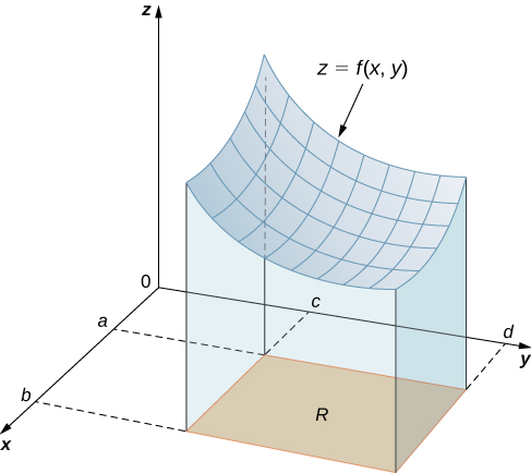
Here [ a , b ] × [ c , d ] denotes the Cartesian product of the two closed intervals [ a , b ] and [ c , d ] . It consists of rectangular pairs ( x , y ) such that a x b and c y d . The graph of f represents a surface above the x y -plane with equation z = f ( x , y ) where z is the height of the surface at the point ( x , y ) . Let S be the solid that lies above R and under the graph of f ( [link] ). The base of the solid is the rectangle R in the x y -plane. We want to find the volume V of the solid S .

In xyz space, there is a surface z = f(x, y). On the x axis, the lines denoting a and b are drawn; on the y axis the lines for c and d are drawn. When the surface is projected onto the xy plane, it forms a rectangle with corners (a, c), (a, d), (b, c), and (b, d).
The graph of f ( x , y ) over the rectangle R in the x y -plane is a curved surface.

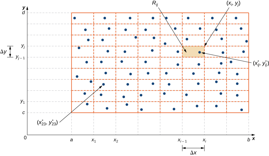
We divide the region R into small rectangles R i j , each with area Δ A and with sides Δ x and Δ y ( [link] ). We do this by dividing the interval [ a , b ] into m subintervals and dividing the interval [ c , d ] into n subintervals. Hence Δ x = b a m , Δ y = d c n , and Δ A = Δ x Δ y .

In the xy plane, there is a rectangle with corners (a, c), (a, d), (b, c), and (b, d). Between a and b on the x axis lines are drawn from a, x1, x2, …, xi, …, b with distance Delta x between each line; between c and d on the y axis lines are drawn from c, y1, y2, …, yj, …, d with distance Delta y between each line. Among the resulting subrectangles, the one in the second column and third row up has a point marked (x*23, y*23). The rectangle Rij is marked with upper right corner (xi, yj). Within this rectangle the point (x*ij, y*ij) is marked.
Rectangle R is divided into small rectangles R i j , each with area Δ A .

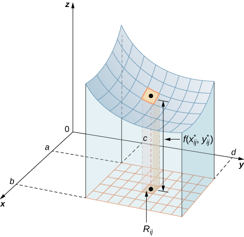
The volume of a thin rectangular box above R i j is f ( x i j * , y i j * ) Δ A , where ( x i j * , y i j * ) is an arbitrary sample point in each R i j as shown in the following figure.

In xyz space, there is a surface z = f(x, y). On the x axis, the lines denoting a and b are drawn; on the y axis the lines for c and d are drawn. When the surface is projected onto the xy plane, it forms a rectangle with corners (a, c), (a, d), (b, c), and (b, d). There are additional squares drawn to correspond to changes of Delta x and Delta y. On the surface, a square is marked and its projection onto the plane is marked as Rij. The average value for this small square is f(x*ij, y*ij).
A thin rectangular box above R i j with height f ( x i j * , y i j * ) .

Using the same idea for all the subrectangles, we obtain an approximate volume of the solid S as V i = 1 m j = 1 n f ( x i j * , y i j * ) Δ A . This sum is known as a double Riemann sum    and can be used to approximate the value of the volume of the solid. Here the double sum means that for each subrectangle we evaluate the function at the chosen point, multiply by the area of each rectangle, and then add all the results.

As we have seen in the single-variable case, we obtain a better approximation to the actual volume if m and n become larger.

V = lim m , n i = 1 m j = 1 n f ( x i j * , y i j * ) Δ A or V = lim Δ x , Δ y 0 i = 1 m j = 1 n f ( x i j * , y i j * ) Δ A .

Note that the sum approaches a limit in either case and the limit is the volume of the solid with the base R . Now we are ready to define the double integral.

Definition

The double integral    of the function f ( x , y ) over the rectangular region R in the x y -plane is defined as

R f ( x , y ) d A = lim m , n i = 1 m j = 1 n f ( x i j * , y i j * ) Δ A .

If f ( x , y ) 0 , then the volume V of the solid S , which lies above R in the x y -plane and under the graph of f , is the double integral of the function f ( x , y ) over the rectangle R . If the function is ever negative, then the double integral can be considered a “signed” volume in a manner similar to the way we defined net signed area in The Definite Integral .

Practice Key Terms 4

Get Jobilize Job Search Mobile App in your pocket Now!

Get it on Google Play Download on the App Store Now


Source:  OpenStax, Calculus volume 3. OpenStax CNX. Feb 05, 2016 Download for free at http://legacy.cnx.org/content/col11966/1.2
Google Play and the Google Play logo are trademarks of Google Inc.

Notification Switch

Would you like to follow the 'Calculus volume 3' conversation and receive update notifications?

Ask