| << Chapter < Page | Chapter >> Page > |
The base case of the recursion are lists of size zero or one, which are always sorted. The algorithm always terminates because it puts at least one element in its final place on each iteration (the loop invariant).
In simple pseudocode , the algorithm might be expressed as:
function quicksort(array)
var list less, pivotList, greater
if length(array) ≤ 1
return array
select a pivot value pivot from array
for each x in array
if x<pivot then add x to less
if x = pivot then add x to pivotList
if x>pivot then add x to greater
return concatenate(quicksort(less), pivotList, quicksort(greater))
Notice that we only examine elements by comparing them to other elements. This makes quicksort a comparison sort .

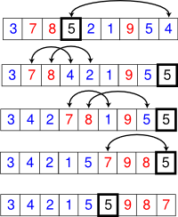
In-place partition in action on a small list. The boxed element is the pivot element, blue elements are less or equal, and red elements are larger.
The disadvantage of the simple version above is that it requires Ω(n) extra storage space, which is as bad as mergesort (see big-O notation for the meaning of Ω). The additional memory allocations required can also drastically impact speed and cache performance in practical implementations. There is a more complicated version which uses an in-place partition algorithm and can achieve O(log n) space use on average for good pivot choices:
function partition(array, left, right, pivotIndex)
pivotValue := array[pivotIndex]
swap( array, pivotIndex, right) // Move pivot to end
storeIndex := left - 1
for i from left to right-1
if array[i]<= pivotValue
storeIndex := storeIndex + 1
swap( array, storeIndex, i)
swap( array, right, storeIndex+1) // Move pivot to its final place
return storeIndex+1
This form of the partition algorithm is not the original form; multiple variations can be found in various textbooks, such as versions not having the storeIndex. However, this form is probably the easiest to understand.
This is the in-place partition algorithm. It partitions the portion of the array between indexes left and right, inclusively, by moving all elements less than or equal to a[pivotIndex] to the beginning of the subarray, leaving all the greater elements following them. In the process it also finds the final position for the pivot element, which it returns. It temporarily moves the pivot element to the end of the subarray, so that it doesn't get in the way. Because it only uses exchanges, the final list has the same elements as the original list. Notice that an element may be exchanged multiple times before reaching its final place.
Once we have this, writing quicksort itself is easy:
function quicksort(array, left, right)
if right>left
select a pivot index (e.g. pivotIndex := left)
pivotNewIndex := partition(array, left, right, pivotIndex)
quicksort(array, left, pivotNewIndex-1)
quicksort(array, pivotNewIndex+1, right)
Like
mergesort , quicksort can also be easily
parallelized due to its divide-and-conquer nature. Individual in-place partition operations are difficult to parallelize, but once divided, different sections of the list can be sorted in parallel. If we have p processors, we can divide a list of n elements into p sublists in Θ(n) average time, then sort each of these in
![]() average time. Ignoring the O(n) preprocessing, this is
linear speedup . Given Θ(n) processors, only O(n) time is required overall.
average time. Ignoring the O(n) preprocessing, this is
linear speedup . Given Θ(n) processors, only O(n) time is required overall.

Notification Switch
Would you like to follow the 'Data structures and algorithms' conversation and receive update notifications?