| << Chapter < Page | Chapter >> Page > |
Although these identities apply to the products of sine and cosine values for single angles a and b , it is a simple matter to extend them to represent the products of time series consisting of sine andcosine functions. Such an extension is shown in Figure 8 .
In each of the three cases shown in Figure 8 , the function f(n) is a time series produced by multiplying two other time series, which are either sinefunctions or cosine functions.
| Figure 8. Products of sine and cosine functions. |
|---|
1. f(n) = sin(a*n)*sin(b*n) =
          (1/2)*(cos((a-b)*n)-cos((a+b)*n))2. f(n) = cos(a*n)*cos(b*n) =
          (1/2)*(cos((a-b)*n)+cos((a+b)*n))3. f(n) = sin(a*n)*cos(b*n) =
(1/2)*(sin((a+b)*n)+sin((a-b)*n)) |
Figure 9 rewrites and simplifies these three functions for the special case where a=b , taking into account the fact that cos(0) =1 and sin(0) = 0.
| Figure 9. Rewrite and simplify. |
|---|
1. f(n) = sin(a*n)*sin(a*n) = (1/2)-cos(2*a*n)/2
2. f(n) = cos(a*n)*cos(a*n) = (1/2)+cos(2*a*n)/23. f(n) = sin(a*n)*cos(a*n) = sin(2*a*n)/2 |
First you need to recall that the average of the values describing any true sinusoid is zero when the average is computed over an even number of cycles ofthe sinusoid.
(A true sinusoid does not have a bias to prevent it from being centered on the horizontal axis.)
If a time series consists of the sum of two true sinusoids, then the average of the values describing that time series will be zero if the average iscomputed over an even number of cycles of both sinusoids, and very close to zero if the average is computed over a period that is not an even number of cyclesfor either or both sinusoids.
(The average will approach zero as the length of data over which the average is computed increases.)
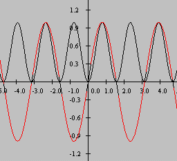
Let's apply this knowledge to the three cases shown above for a=b . Consider the time series for case 1 in Figure 9 . This case is the product of two sine functions having the same frequency. The result of multiplying the two sinefunctions is shown graphically in Figure 10 .
| Figure 10. Plot of sin(x) and sin(x)*sin(x). |
|---|
 |
The red curve in Figure 10 shows the function sin(x), and the black curve shows the function produced by multiplying sin(x) by sin(x).
If you sum the values of the black curve over an even number of cycles, the sum will not be zero. Rather, it will be a positive, non-zero value.
Now refer back to Imag(F) in Figure 6 . The imaginary part is computed by multiplying the time series by a sine function and computing the sum of theproducts. If that time series contains a sine component with the same frequency as the sine function, that component will contribute a non-zero value to the sumof products. Thus, the imaginary part of the transform at that frequency will not be zero.
Now consider the time series for case 2 in Figure 9 . This case is the product of two cosine functions having the same frequency. The result of multiplying twocosine functions having the same frequency is shown graphically in Figure 11 .

Notification Switch
Would you like to follow the 'Digital signal processing - dsp' conversation and receive update notifications?