| << Chapter < Page | Chapter >> Page > |
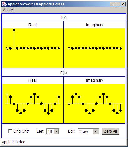
The shape of the imaginary part of the transform is an upside down sine curve.
This transform program computes real and imaginary values from zero to an output index that is one output sample interval less than the samplingfrequency. The number of output values is equal to the number of samples in the input series. This is very typical of FFT algorithms.
In this case, I set the applet up to accept sixteen input samples and to produce sixteen output samples.
For the moment, lets think in terms of time and frequency. Assume that the input series f(x) is a time series and the output series F(k) is a frequencyspectrum.
To make the arithmetic easy, let's assume that the sampling interval for the input time series in the upper left box of Figure 5 is one second. This gives a sampling frequency of one sample per second, and a total elapsed time of sixteenseconds.
The sine and cosine curves in Figure 5 each go through one complete period between a frequency of zero and the sampling frequency, which one sample persecond. Thus, the period of the sine and cosine curves along the frequency axis is one sample per second. This is the reciprocal of the time shift of one sampleinterval at a sampling frequency of one sample per second.
Stated differently, the number of periods of the sine and cosine curves in the real and imaginary parts of the transform between a frequency of zero and afrequency equal to the sampling frequency is equal to the shift in sample intervals. A shift of one sample interval produces sine and cosine curves havingone period in the frequency range from zero to the sampling frequency. A shift of two sample intervals produces sine and cosine curves having two periods inthe frequency range from zero to the sampling frequency, etc. This is illustrated by Figure 6 .
Figure 6 shows the transform of an impulse with a shift equal to two sample intervals and a positive value.
| Figure 6. Transform of an impulse with a shift equal to two sample intervals and a positive value. |
|---|
 |
The real part of the transform has the shape of a cosine curve with two complete periods between zero and an output index equal to the samplingfrequency.
The imaginary part of the transform has the shape of a sine curve with two complete periods within the same output interval. This agrees with theconclusions stated in the previous section.
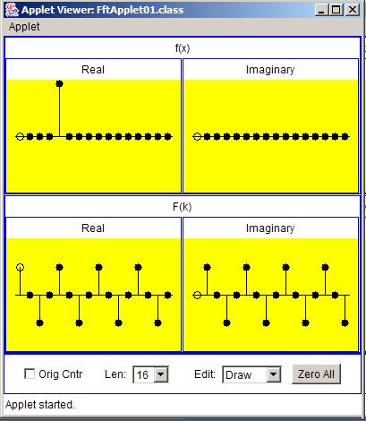
Finally, Figure 7 shows the transform of an impulse with a shift equal to four sample intervals.
| Figure 7. Transform of an impulse with a shift equal to four sample intervals and a positive value. |
|---|
 |
The cosine and sine curves that represent the real and imaginary parts of the transform each have four complete periods between zero and an output index equalto the sampling frequency.
In this case the cosine and sine curves are very sparsely sampled.
The main point is:

Notification Switch
Would you like to follow the 'Digital signal processing - dsp' conversation and receive update notifications?