| << Chapter < Page | Chapter >> Page > |
(Note however, that you may not see the zero-valued points in the spectrum if you don't compute the spectral values at exactly those frequencyvalues. This is the case for some of the plots in Figure 11 .)
Some analysts regard a frequency interval equal to the reciprocal of the length of the time series as being the useful resolution of the spectrumanalysis process.
In other words, two peaks in the spectrum cannot be resolved if the frequency difference between them is less than the reciprocal of the length of the timeseries.
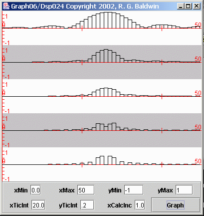
This is illustrated by the plots in Figure 15 . Figure 15 is similar to Figure 13 with one major difference. In Figure 13 , the frequency difference between the two sinusoids that made up each of the time series was rather large. In Figure 15 , the frequency difference between the two sinusoids that made up each of the time series was reduced to 1/400, (the reciprocal of the length of the longest time series).
| Figure 15. Illustration of frequency resolution. |
|---|
 |
Each plot in Figure 15 shows the first 50 points produced by performing a Fourier transform on one of the time series. In each case, the time seriesconsisted of the sum of two sinusoids with a frequency separation of 1/400.
The length of the time series for the bottom plot was 400 samples. Thus, the separation of the two sinusoids matched the frequency resolution available by performing a Fourier transform on that time series.
As you can see, the two peaks in the spectrum were resolved by the bottom plot in Figure 15 .
The other four time series were shorter, having lengths of 80, 160, 240, and 320 samples respectively, from top to bottom.
The important thing to note in Figure 15 is that the spectrum analysis performed on the 400-sample time series was successful in separating the twopeaks.
However, even though the spectrum analysis on the 320-sample time series hinted at a separation of the peaks, none of the spectrum analyses on the timeseries that were shorter than 400 samples successfully separated the peaks.
This illustrates that the frequency resolution of the Fourier transform is the reciprocal of the length of the time series.
I'm going to show you one more picture and then call it a wrap for this module. Figure 16 is similar to Figure 15 with one major difference.
| Figure 16. Illustration of frequency resolution. |
|---|
 |
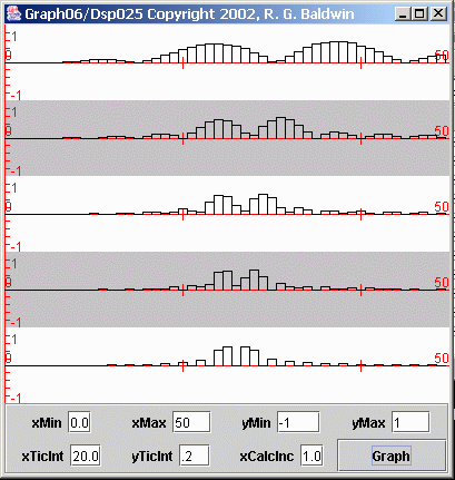
As before, the five plots in Figure 16 show the first 50 points produced by performing a Fourier transform on five different time series. Starting at thetop, the lengths of the time series were 80, 160, 240, 320, and 400 samples.
Also as before, each time series was the sum of two sinusoids with closely-spaced frequencies. However, in Figure 16 , the difference between the sinusoidal frequencies was different from one time series to the next.
In Figure 16 , the frequency difference for the sinusoids contained in each time series was the reciprocal of the length of that particular time series.Therefore, the frequency difference for each case matched the frequency resolution of the Fourier transform.
The frequency of the lower-frequency peak was the same in all five cases. Therefore, this peak should line up vertically for the five plots in Figure 16 .
The frequency difference between the sinusoids was achieved by increasing the higher frequency by an amount equal to the reciprocal of the length of the timeseries.
If you examine Figure 16 , you will see that the peaks corresponding to the two sinusoids were resolved for all five time series.
As would be expected, the peaks appear to be broader for the shorter time series having the lower frequency resolution. The peaks are also separated inall five cases. However, the peaks for the lower-frequency sinusoid don't exactly line up vertically. Thus we see a small amount of measurement error inthe positions of the peaks
This module has presented a pseudo-mathematical discussion of issues involving the averaging of time series, and the impact of those issues onspectrum analysis.
Those averaging issues have an impact on many other areas of DSP as well, but the detrimental effect is probably more obvious in spectrum analysis than in otherareas.
This section contains a variety of miscellaneous information.
Baldwin begins with a discussion of averaging time series, and ends with a discussion of spectral resolution, covering several related topics in between.
Financial : Although the Connexions site makes it possible for you to download a PDF file for thismodule at no charge, and also makes it possible for you to purchase a pre-printed version of the PDF file, you should beaware that some of the HTML elements in this module may not translate well into PDF.
I also want you to know that, I receive no financial compensation from the Connexions website even if you purchase the PDF version of the module.
In the past, unknown individuals have copied my modules from cnx.org, converted them to Kindle books, and placed them for sale on Amazon.com showing me as the author. Ineither receive compensation for those sales nor do I know who does receive compensation. If you purchase such a book, please beaware that it is a copy of a module that is freely available on cnx.org and that it was made and published withoutmy prior knowledge.
Affiliation : I am a professor of Computer Information Technology at Austin Community College in Austin, TX.
-end-

Notification Switch
Would you like to follow the 'Digital signal processing - dsp' conversation and receive update notifications?