| << Chapter < Page | Chapter >> Page > |
A “row matrix” means a matrix with only one row. A “column matrix” means a matrix with only one column. When a row matrix has the same number of elements as a column matrix, they can be multiplied. So the following is a perfectly legal matrix multiplication problem:
These two matrices could not be added, of course, since their dimensions are different, but they can be multiplied. Here’s how you do it. You multiply the first (left-most) item in the row, by the first (top) item in the column. Then you do the same for the second items, and the third items, and so on. Finally, you add all these products to produce the final number.

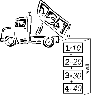
A couple of my students (Nakisa Asefnia and Laura Parks) came up with an ingenious trick for visualizing this process. Think of the row as a dump truck, backing up to the column dumpster. When the row dumps its load, the numbers line up with the corresponding numbers in the column, like so:

So, without the trucks and dumpsters, we express the result—a row matrix, times a column matrix—like this:
There are several subtleties to note about this operation.
It’s important to practice a few of these, and get the hang of it, before you move on.
The general algorithm for multiplying matrices is built on the row-times-column operation discussed above. Consider the following example:
The key to such a problem is to think of the first matrix as a list of rows (in this case, 4 rows), and the second matrix as a list of columns (in this case, 2 columns). You are going to multiply each row in the first matrix, by each column in the second matrix. In each case, you will use the “dump truck” method illustrated above.
Start at the beginning: first row, times first column.
Now, move down to the next row. As you do so, move down in the answer matrix as well.
Now, move down the rows in the first matrix, multiplying each one by that same column on the right. List the numbers below each other.
The first column of the second matrix has become the first column of the answer. We now move on to the second column and repeat the entire process, starting with the first row.
And so on, working our way once again through all the rows in the first matrix.
We’re done. We can summarize the results of this entire operation as follows:
It’s a strange and ugly process—but everything we’re going to do in the rest of this unit builds on this, so it’s vital to be comfortable with this process. The only way to become comfortable with this process is to do it. A lot. Multiply a lot of matrices until you are confident in the steps.
Note that we could add more rows to the first matrix, and that would add more rows to the answer. We could add more columns to the second matrix, and that would add more columns to the answer. However—if we added a column to the first matrix, or added a row to the second matrix, we would have an illegal multiplication. As an example, consider what happens if we try to do this multiplication in reverse:
Illegal multiplication
If we attempt to multiply these two matrices, we start (as always) with the first row of the first matrix, times the first column of the second matrix: . But this is an illegal multiplication; the items don’t line up, since there are two elements in the row and four in the column. So you cannot multiply these two matrices.
This example illustrates two vital properties of matrix multiplication.

Notification Switch
Would you like to follow the 'Advanced algebra ii: conceptual explanations' conversation and receive update notifications?