| << Chapter < Page | Chapter >> Page > |
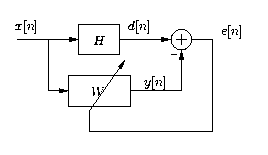
[link] is a block diagram of system identification using adaptive filtering. The objective is tochange (adapt) the coefficients of an FIR filter, , to match as closely as possible the response of an unknown system, . The unknown system and the adapting filter process the same input signal and have outputs (also referred to as the desired signal) and .

The adaptive filter, , is adapted using the least mean-square algorithm, which is the most widely used adaptive filteringalgorithm. First the error signal, , is computed as , which measures the difference between the output of the adaptive filter and the output of the unknown system.On the basis of this measure, the adaptive filter will change its coefficients in an attempt to reduce the error.The coefficient update relation is a function of the error signal squared and is given by
The term inside the parentheses represents the gradient of the squared-error with respect to the coefficient. The gradient is a vector pointing in the direction of the change in filter coefficients that willcause the greatest increase in the error signal. Because the goal is to minimize the error, however, [link] updates the filter coefficients in the direction opposite the gradient; that is why the gradientterm is negated. The constant is a step-size, which controls the amount of gradient information used to update each coefficient. Afterrepeatedly adjusting each coefficient in the direction opposite to the gradient of the error, the adaptive filtershould converge; that is, the difference between the unknown and adaptive systems should get smaller and smaller.
To express the gradient decent coefficient update equation in a more usable manner, we can rewrite the derivative of thesquared-error term as
Simulate the system identification block diagram shown in [link] .
Previously in MATLAB, you used the
filter command
or the
conv command to implement shift-invariant
filters. Those commands will not work here because adaptivefilters are shift-varying, since the coefficient update
equation changes the filter's impulse response at every sampletime. Therefore, implement the system identification block on
a sample-by-sample basis with a
do loop, similar
to the way you might implement a time-domain FIR filter on aDSP. For the "unknown" system, use the fourth-order,
low-pass, elliptical, IIR filter designed for the
IIR Filtering: Filter-Design Exercise in
MATLAB .
Use Gaussian random noise as your input, which can be
generated in MATLAB using the command
randn .
Random white noise provides signal at all digital frequenciesto train the adaptive filter. Simulate the system with an
adaptive filter of length 32 and a step-size of
. Initialize all of the adaptive filter coefficients
to zero. From your simulation, plot the error (orsquared-error) as it evolves over time and plot the frequency
response of the adaptive filter coefficients at the end of thesimulation. How well does your adaptive filter match the
"unknown" filter? How long does it take to converge?
Once your simulation is working, experiment with different step-sizes and adaptive filter lengths.
Use the same "unknown" filter as you used in the MATLAB simulation.
Although the coefficient update equation is relatively
straightforward, consider using the
lms instruction available on the TI processor, which is designed
for this application and yields a very efficientimplementation of the coefficient update equation.
To generate noise on the DSP, you can use the PN generator from the Digital Transmitter: Introduction to Quadrature Phase-Shift Keying , but shift the PN register contents up to make the sign bit random.(If the sign bit is always zero, then the noise will not be zero-mean and this will affect convergence.) Send the desiredsignal, , the output of the adaptive filter, , and the error to the D/A for display on the oscilloscope.
When using the step-size suggested in the MATLAB simulation section, you should notice that the error converges veryquickly. Try an extremely small so that you can actually watch the amplitude of the error signal decrease towards zero.
If your project requires some modifications to the implementation here, refer to Haykin and consider some of the following questions regarding such modifications:

Notification Switch
Would you like to follow the 'Dsp laboratory with ti tms320c54x' conversation and receive update notifications?