| << Chapter < Page | Chapter >> Page > |
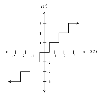
Quantization can be thought of as a functional mapping of a real-valued input to a discrete-valued output. An example of a quantization function is shown in [link] , where the x-axis is the input value, and the y-axis is the quantizedoutput value.

Quantization is sometimes used for compression. As an example, suppose we have a digital image which isrepresented by 8 different gray levels: [0 31 63 95 159 191 223 255].To directly store each of the image values, we need at least 8-bits for each pixel since the values range from 0 to 255.However, since the image only takes on 8 different values, we can assign a different 3-bit integer (a code) to represent each pixel:[000 001 ... 111].Then, instead of storing the actual gray levels, we can store the 3-bit code for each pixel.A look-up table, possibly stored at the beginning of the file, would be used to decode the image.This lowers the cost of an image considerably: less hard drive space is needed, and less bandwidth is required to transmit the image (i.e. itdownloads quicker). In practice, there are much more sophisticated methods of compressing imageswhich rely on quantization.
Download the file fountainbw.tif for the following section.
The image in
fountainbw.tif is an 8-bit grayscale image.
We will investigate what happens when we quantize it to fewer bitsper pixel (b/pel).
Load it into Matlab and display it using the following sequence ofcommands:
y = imread('fountainbw.tif');
image(y);
colormap(gray(256));
axis('image');
The image array will initially be of type
uint8 , so you
will need to convert the image matrix to type
double before performing any computation.
Use the command
z=double(y) for this.
There is an easy way to uniformly quantize a signal. Let
where X is the signal to be quantized, and N is the number of quantization levels.To force the data to have a uniform quantization step of ,
Write a Matlab function
Y = Uquant(X,N) which will
uniformly quantize an input array
(either a vector or a matrix)
to
discrete levels.
Use this function to quantize the fountain image to7 b/pel, 6, 5, 4, 3, 2, 1 b/pel, and observe the output images.
Download the files speech.au and music.au for the following section.
If an audio signal is to be coded, either for compression or for digital transmission, it must undergo some form of quantization.Most often, a general technique known as vector quantization is employed for this task, but this technique must be tailored to thespecific application so it will not be addressed here. In this exercise, we will observe the effect of uniformlyquantizing the samples of two audio signals.

Notification Switch
Would you like to follow the 'Purdue digital signal processing labs (ece 438)' conversation and receive update notifications?