| << Chapter < Page | Chapter >> Page > |
As mentioned earlier, the DFT algorithm is much more flexible while the FFT algorithm is much faster, particularly for large data lengths.
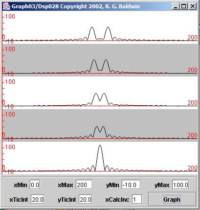
In addition to illustrating these fundamental aspects of the DFT algorithm, this example also illustrates how the mirror image peaks on either side of thefolding frequency merge into a single larger peak as the data frequency approaches the folding frequency.
The input parameters are shown in Figure 10 . Note in particular the values for the following parameters:
| Figure 10. The input parameters. |
|---|
Data length: 200
Sample for zero time: 0Lower frequency bound: 0.4
Upper frequency bound: 0.6Number spectra: 5
Frequencies0.492
0.4940.496
0.4980.5
Amplitudes90.0
90.090.0
90.090.0 |
As you can see, the data length for this experiment is different from the data length of 400 used earlier. In addition, neither data length is a power oftwo.
As you can also see, the lower and upper frequency bounds are not 0.0 and 1.0 as in the earlier cases. In this case, the frequency bounds describe a muchnarrower range centered on the folding frequency.
Finally, the frequencies of each of the five sinusoids specified in Figure 10 is progressively closer to the folding frequency with the frequency of the fifthsinusoid being equal to the folding frequency.
The output from the spectral analysis for each of the five sinusoids is shown in Figure 11 . (Another interesting view of the same results is shown later in Figure 14 .)
| Figure 11. Spectral analysis of five sinusoids. |
|---|
 |
The spectral peaks shown in Figure 11 are symmetrical about the folding frequency, which in turn is centered horizontally in each of the graphs. As youalready know, the peaks are always symmetrical about the folding frequency due to the frequency folding at that frequency.
The folding frequency is centered horizontally due to the way that I defined the lower and upper frequency bounds, and the way that I adjusted the plottingparameters.
The peaks are well defined because I computed the spectral energy at 200 points across the specified frequency range from 0.4 to 0.6. Thus, the frequencybins at which I computed spectral energy were much narrower than before.
The peaks are wider because I displayed a much smaller slice of the entire frequency spectrum in the same physical screen space.
As the frequency of each sinusoid approaches the folding frequency, the two mirror-image peaks corresponding to that sinusoid merge into a single peak withtwice the height at the folding frequency. This agrees with what you saw in Figure 9 , but on a much more detailed basis.
It would be difficult to perform this experiment using an FFT algorithm because of the inherent limitations built into the algorithm. The FFT algorithmsacrifices flexibility for speed.

Notification Switch
Would you like to follow the 'Digital signal processing - dsp' conversation and receive update notifications?