| << Chapter < Page | Chapter >> Page > |
(As mentioned earlier, this process would work even if the time series contained sinusoids other than cosine functions. However, the explanationwould be more complicated.)
Every other sinusoidal component in the time series (whose frequency doesn't match the selected frequency), will produce a new time series containing two sinusoids when multiplied by the sine function or the cosinefunction.
The frequency of one of the sinusoids in the new time series will be the sum of the frequencies of the sinusoidal component and the sine or cosine function.The frequency of the other sinusoid will be the difference in the frequencies between the sinusoidal component and the sine or cosine function.
As you saw earlier, when this difference is very small, the frequency of the new sinusoid will be very near to zero.
Ideally, the average value of the product should be zero when the frequency of the original sinusoidal component is different from the sine or cosinefunction by which it is multiplied. The computed average of this time series will converge on zero with the quality of the estimate depending on the numberof points in the average.
However, (and this is very important), when the frequency of the original sinusoid is very close to the frequency of the sine or cosine function,the convergence on zero will be poor even for a large number of points in the average.
Thus, the computation at those frequencies very near to the frequency of an actual sinusoidal component in the raw data will produce a non-zeroaverage value even when there is no sinusoidal component in the raw data at those frequencies. This is a form of measurement error.
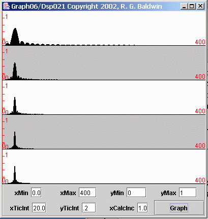
With that as a preface, lets look at some graphs ( Figure 10 and Figure 11 ) resulting from spectral analyses. (These two figures show two different views of the same data.)
| Figure 10. Spectra of five different sinusoids of different lengths. |
|---|
 |
Figure 10 shows the individual spectra computed for five different sinusoids, each having the same frequency, but different lengths. The combination ofsampling rate and frequency was such that each sinusoid had 32 samples per cycle.
Starting at the top in Figure 10 , the lengths of the five sinusoids were 80, 160, 240, 320, and 400 samples. (The lengths of the five sinusoids were multiples of 80 samples.)
As mentioned earlier, for the cases where the actual length of the sinusoid was less than 400 samples, the length was extended to 400 samples by appendingan appropriate number of samples having zero values.
(This made it easy to compute and plot the spectrum for every sinusoid over the same frequency range with the same number of points in each plot.)
The spectrum was computed and plotted for each sinusoid at 400 individual frequency points between zero and the folding frequency.
Even though the Fourier transform program averaged across 400 samples in all cases, the effective averaging length was equal to the length of the sinusoid. All product points outside that length had a value of zero andcontributed nothing to the average one way or the other.

Notification Switch
Would you like to follow the 'Digital signal processing - dsp' conversation and receive update notifications?