| << Chapter < Page | Chapter >> Page > |
In this expression, the noise is the error signal
E .
Generally, this means that a higher PSNR implies a less noisy signal.
From previous labs we know the power of a sampled signal, , is defined by
where is the length of . Compute the PSNR for the four quantized speech signals from the previoussection.
In evaluating quantization (or compression) algorithms, a graph called a “rate-distortion curve" is often used.This curve plots signal distortion vs. bit rate . Here, we can measure the distortion by , and determine the bit rate from the number of quantization levels and sampling rate.For example, if the sampling rate is 8000 samples/sec, and we are using 7 bits/sample, the bit rate is 56 kilobits/sec (kbps).
Assuming that the speech is sampled at 8kHz, plot the rate distortion curve using as the measure of distortion.Generate this curve by computing the PSNR for 7, 6, 5,..., 1 bits/sample. Make sure the axes of the graphare in terms of distortion and bit rate .
In this section, we will investigate a different type of quantizer which produces less noise for a fixed number of quantization levels.As an example, let's assume the input range for our signal is [-1,1], but most of the input signal takes on values between [-0.2, 0.2]. If we place more of the quantizationlevels closer to zero, we can lower the average error due to quantization.
A common measure of quantization error is mean squared error (noise power). The Max quantizer is designed to minimize the mean squared error for a given set of training data.We will study how the Max quantizer works, and compare its performance to that of the uniform quantizer which was used in the previoussections.
The Max quantizer determines quantization levels based on a data set's probability density function, , and the number of desired levels, . It minimizes the mean squared error between the originaland quantized signals:
where is the quantization level, and is the lower boundary for . The error depends on both and . (Note that for the Gaussian distribution, , and .) To minimize with respect to , we must take and solve for :
We still need the quantization boundaries, . Solving yields:
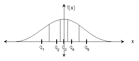
This means that each non-infinite boundary is exactly halfway in between the two adjacent quantization levels, and that eachquantization level is at the centroid of its region. [link] shows a five-level quantizer for a Gaussian distributed signal. Note that the levels are closer together in areas of higher probability.

Download the file speech.au for the following section.
In this section we will use Matlab to compute an optimal quantizer, and compare its performance to the uniform quantizer.Since we almost never know the actual probability density function of the data that the quantizer will be applied to,we cannot use equation [link] to compute the optimal quantization levels.Therefore, a numerical optimization procedure is used on a training set of data to compute the quantization levels and boundaries which yield the smallest possible error for that set.
Matlab has a built-in function called
lloyds which performs
this optimization.It's syntax is...
[partition, codebook] = lloyds(training_set, initial_codebook);
This function requires two inputs. The first is the training data set, from which it will estimatethe probability density function. The second is a vector containing an initial guess of theoptimal quantization levels. It returns the computed optimalboundaries (the “partition”) and quantization levels (the “codebook”).
Since this algorithm minimizes the error with respect to the quantization levels, it is necessary to provide a decent initial guess of the codebook to help ensure a valid result. If the initial codebook is significantly “far" away from the optimalsolution, it's possible that the optimization will get trapped in a local minimum, and the resultant codebook may perform quite poorly.In order to make a good guess, we may first estimate the shape of the probability density function of the training set usinga histogram. The idea is to divide the histogram into equal “areas" and choosequantization levels as the centers of each of these segments.
First plot a 40-bin histogram of this speech signal using
hist(speech,40) , and make an initial guess of
the four optimal quantization levels.Print out the histogram.
Then use the
lloyds function to compute an optimal 4-level
codebook using
speech.au as the training set.
Once the optimal codebook is obtained, use the codebook and partition vectors to quantize the speech signal. This may be done with a for loop and if statements. Then compute the error signal and PSNR.On the histogram plot, mark where the optimal quantization levels fall along the x-axis.

Notification Switch
Would you like to follow the 'Purdue digital signal processing labs (ece 438)' conversation and receive update notifications?