| << Chapter < Page | Chapter >> Page > |
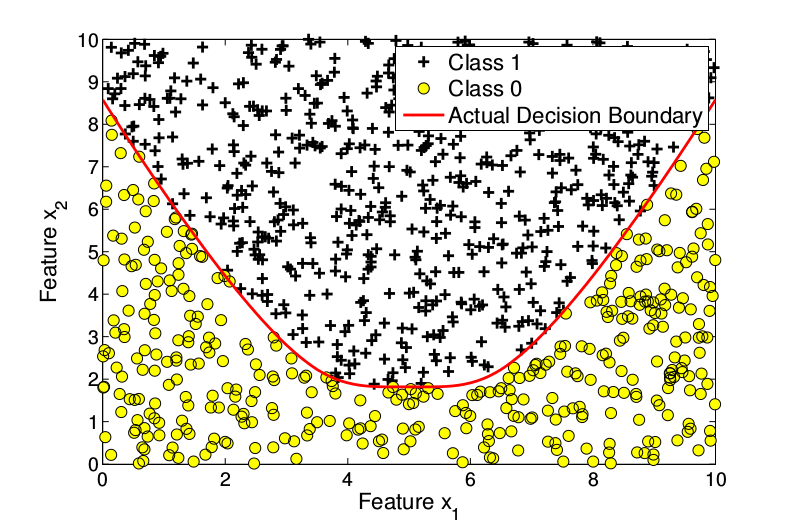
The figure below plots the training data and the actual decision boundary.

We split the training data set into 3 separate sets, training set with 600 examples, cross-validation set with 200 examples and test data set with 200 examples.
This training data was then fed into a logistic regression classifier to study the performance of the classifier. It is important to note that the objective of logistic regression classifier is maximizing the accuracy of labeling the data into two classes. Unlike linear regression, the decision boundary of the logistic regression classifier does not try to match the underlying true boundary which divides the data into two classes.
In addition to the two features that identify a training example, polynomial features up to a desired degree are generated. We start off the optimization with an initial parameter value of all 0. The optimization of the cost function is done using the Matlab's built-in fminunc function. A function costFunctionReg.m that outputs the regularized cost and regularized gradient, with the training data, parameter values and the regularization parameter as inputs, is given as input along with initial parameter values to this fminunc function.
Now we vary the maximum degree of the polynomial features to study the decision boundary of the classifier. Its important to note that the values of the parameters are obtained from the training data set, for a given value of maximum degree. The optimal values of maximum degree are determined by the performance on the cross-validation set. Finally, the decision boundary obtained by solving for the parameters with optimal values of maximum degree is used to evaluate the performance on a test data set, in order to see how well the classifier generalizes.
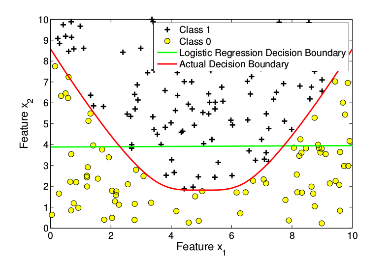
The decision boundary for a degree 1 polynomial is shown in [link] below. The accuracy on the cross-validation set was .

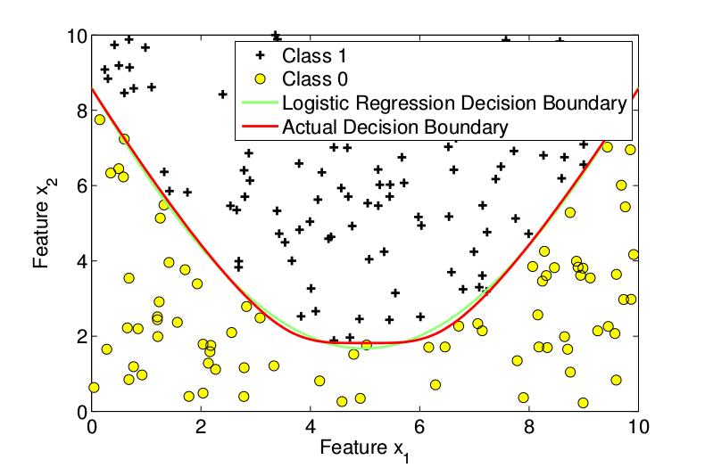
From [link] it is clear that 1 st degree features are not sufficient to capture both classes. So the maximum degree was increased to 2. [link] plots the decision boundary for degree 2. The accuracy of the classifier on cross-validation set in this case was .

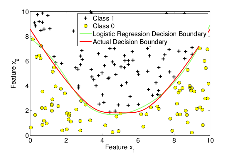
We now try the maximum degree of 3. [link] plots the decision boundary with maximum degree 3. The accuracy on cross-validation set is 98.00.

Due to its lower accuracy, the logistic regression classifier with maximum degree 2 is chosen from amongst the 3 classifiers. This classifier was then evaluated on test data set to study how well it generalizes. The accuracy of this classifier on test set was 98.00. Hence this logistic regression classifier generalizes very well.
To see the MATLAB code that generated these plots, download the following .zip file: MATLAB files for simulated data. !
As was stated, this collection is intended to be an introduction to regression analysis, but is sufficient in order to understand the application of logistic regression to an application. There are plenty of resources to learn more about more nuanced views of the key components of the theory, and more resources to see logistic regression in action!
For an application of Logistic Regression to a synthetic dataset and to a real-world problem in statistical physics, see Optimizing Logistic Regression for Particle Physics !

Notification Switch
Would you like to follow the 'Introductory survey and applications of machine learning methods' conversation and receive update notifications?