<< Chapter < Page
  From matlab and simulink to real     Page 1 / 3
Chapter >> Page >
The Least Mean Squares (LMS) Algorithm can be used in a range of Digital Signal Processing applications such as echo cancellation and acoustic noise reduction. This laboratory shows how to design a model of LMS Noise Cancellation using Simulink and run it on a Texas Instruments C6000 DSP.

Introduction

The Least Mean Squares (LMS) Algorithm can be used in a range of Digital Signal Processing applications such as echo cancellation and acoustic noise reduction.

This laboratory shows how to design a model of LMS Noise Cancellation using Simulink and run it on a Texas Instruments C6000 DSP.

Objectives

  • Design a model of LMS Noise Reduction for the Texas Instruments C6000 family of DSP devices using MATLAB® and Simulink®.
  • Modify an existing Simulink demonstration model for use as a template.
  • Run the project on the Texas Instruments DSK6713 with a microphone and computer loudspeakers / headphones.

Level

Intermediate - Assumes prior knowledge of MATLAB and Simulink. It also requires a theoretical understanding of matrices and the LMS algorithm.

Hardware and software requirements

This laboratory was originally developed using the following hardware and software:

  • MATLAB R2006b with Embedded Target for TI C6000 and the Signal Processing Toolbox.
  • Code Composer Studio (CCS) v3.1
  • Texas Instruments DSK6713 hardware.
  • Microphone and computer loudspeakers / headphones.

Simulation

You will now start with a simple Simulink model and run it to see how it works.

Opening the acoustic noise cancellation model

Open the AcousticNoiseCancellation.mdl
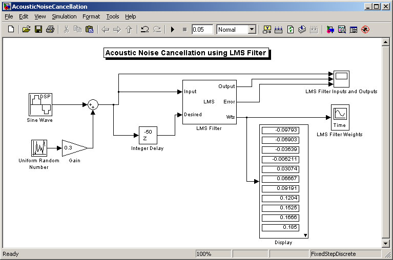
Opening the AcousticNoiseCancellation Model

Run the model.

Inputs and outputs of lms filter

The output from the LMS Filter starts at zero and grows slowly. Initially, some of the sine wave information is lost as LMS Error.

LMS Filter Inputs and Outputs

Lms filter weights (coefficients)

The LMS Filter Weights all start at zero and take several iterations to reach their final values.
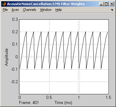
LMS Filter Weights (Coefficients)

Tuning the model

The critical variable in the LMS Filter is the “Step size (mu)”. This sets the rate of convergence of the LMS filter.
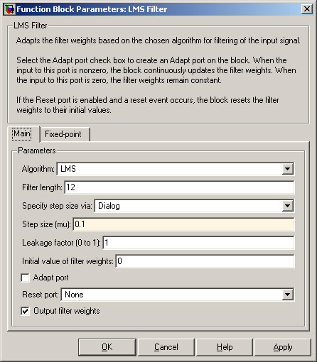
Changing the Step size (mu) to 0.1

Double-click on the “LMS Filter” block and change the “Step size (mu) to 0.1

Run the model.

Filter outputs for step size (mu) = 0.1

When the “Step size (mu)” is increased, LMS algorithm converges more quickly, but at the expense of granularity – the LMS Filter Output is not as smooth.
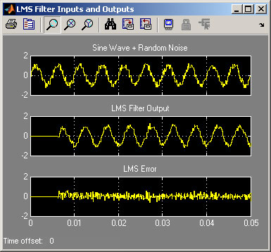
Input and LMS Filter Outputs for Step size (mu) = 0.1

Filter weights for step size (mu) = 0.1

Note that the filter weights (coefficients) do not attain smooth values, as would be the case for smaller values of Step size (mu).
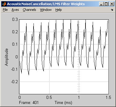
LMS Filter Weights for Step size (mu) = 0.1

Changing the delay

Part of the Acoustic Noise Algorithm is the delay. The delay should ideally be at least half a wavelength so the two inputs to the LMS Filter have different random noise.

Get Jobilize Job Search Mobile App in your pocket Now!

Get it on Google Play Download on the App Store Now


Source:  OpenStax, From matlab and simulink to real-time with ti dsp's. OpenStax CNX. Jun 08, 2009 Download for free at http://cnx.org/content/col10713/1.1
Google Play and the Google Play logo are trademarks of Google Inc.

Notification Switch

Would you like to follow the 'From matlab and simulink to real-time with ti dsp's' conversation and receive update notifications?

Ask